| Home | Blog index | Previous | Next | About | Privacy policy |
By Chris Austin. 28 November 2020.
An earlier version of this post was published on another website on 13 October 2012.
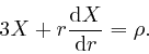
This is the third part of a ten-part post on the foundation of our understanding of high energy physics, which is Richard Feynman's functional integral. The first two parts are Action and Multiple Molecules, and the following parts, which will appear at intervals of about a month, are Action for Fields, Radiation in an Oven, Matrix Multiplication, The Functional Integral, Gauge Invariance, Photons, and Interactions.
I'm hoping this blog will be fun and useful for everyone with an interest in science, so although I'll pop up a few formulae again, I'll still try to keep them friendly by explaining all the pieces, as in the first two parts of the post. Please feel free to ask a question in the Comments, if you think anything in the post is unclear.
The clue that led to the discovery of quantum mechanics, whose principles are summarized in Feynman's functional integral, came from the attempted application to electromagnetic radiation of discoveries about heat and temperature. We looked at those discoveries about heat and temperature in the second part of the post, and today I would like to show you how James Clerk Maxwell, just after the middle of the nineteenth century, was able to identify light as waves of oscillating electric and magnetic fields, and to calculate the speed of light from measurements of:
In addition to his work on the distribution of energy among the molecules in a
gas, which we looked at in the second part
of the post, Maxwell summarized the existing knowledge about electricity
and magnetism into equations now called Maxwell's equations, and after
identifying and correcting a logical inconsistency in these equations, he
showed that they implied the possible existence of waves of oscillating
electric and magnetic fields, whose speed of propagation would be equal within
observational errors to the speed of light, which was roughly known from
Olaf Romer's observation,
made around 1676,
of a 16 minute time lag between the motions of Jupiter's
moons as seen from Earth on the far side of the Sun from Jupiter, and as seen
from Earth on the same side of the Sun as Jupiter, together with the distance
from the Earth to the Sun, which was roughly known from simultaneous
observations of Mars in 1672 from opposite sides of the Atlantic by
Giovanni Domenico Cassini
and Jean Richer, and
observations of the transit of Venus. The speed of light had
also been measured in the laboratory by
Hippolyte Fizeau
in 1849, and more accurately by
Léon Foucault
in 1862. Maxwell therefore suggested that light was electromagnetic
radiation, and that electromagnetic radiation of wavelengths outside the
visible range, which from
Thomas Young's
experiments with double slits was known to comprise wavelengths between about
![]() metres for
violet light and
metres for
violet light and
![]() metres for red light, would also exist.
This was the other part of the clue that led to the discovery of quantum
mechanics and Feynman's functional integral.
metres for red light, would also exist.
This was the other part of the clue that led to the discovery of quantum
mechanics and Feynman's functional integral.
In his writings around 600 BC, Thales of Miletus described how amber attracts light objects after it is rubbed. The Greek word for amber is elektron, which has been adapted to the English word electron, for the first of the elementary matter particles of the Standard Model to be discovered. Benjamin Franklin and Sir William Watson suggested in 1746 that the two types of static electricity, known as vitreous and resinous, corresponded to a surplus and a deficiency of a single "electrical fluid" present in all matter, whose total amount was conserved. Matter with a surplus of the fluid was referred to as "positively" charged, and matter with a deficiency of the fluid was referred to as "negatively" charged. Objects with the same sign of charge repelled each other, and objects with opposite sign of charge attracted each other. Around 1766, Joseph Priestley suggested that the strength of the force between electrostatic charges is inversely proportional to the square of the distance between them, and this was approximately experimentally verified in 1785 by Charles-Augustin de Coulomb, who also showed that the strength of the force between two charges is proportional to the product of the charges.
Most things in the everyday world have no net electric charge, because the charges of the positively and negatively charged particles they contain cancel out. In particular, a wire carrying an electric current usually has no net electric charge, because the charges of the moving particles that produce the current are cancelled by the opposite charges of particles that can vibrate about their average positions, but have no net movement in any direction.
Jean-Baptiste Biot and Félix Savart discovered in 1820 that a steady electric current in a long straight wire produces a magnetic field in the region around the wire, whose direction is at every point perpendicular to the plane defined by the point and the wire, and whose magnitude is proportional to the current in the wire, and inversely proportional to the distance of the point from the wire. André-Marie Ampère discovered in 1826 that this magnetic field produces a force between two long straight parallel wires carrying electric currents, such that the force is attractive if the currents are in the same direction and repulsive if the currents are in opposite directions, and the strength of the force is proportional to the product of the currents, and inversely proportional to the distance between the wires. Thus the force on either wire is proportional to the product of the current in that wire and the magnetic field produced at the position of that wire by the other wire, and the direction of the force is perpendicular both to the magnetic field and the direction of the current.
Ampère's law is used to define both the unit of electric current, which is
called the amp, and the unit of electric charge, which is called the coulomb.
The amp is defined to be the electric current which, flowing along each of
two very long straight parallel thin wires one metre apart in a vacuum,
produces a force of
![]() kilogram metres per second
kilogram metres per second![]() between
them, per metre of their length. The coulomb is then defined to be the
amount of moving electric charge which flows in one second through any
cross-section of a wire carrying a current of one amp. Electric currents are
often measured in practice by moving-coil ammeters, in which the deflection of
the indicator needle is produced by letting the current flow through a movable
coil suspended in the field of a permanent magnet, that has been calibrated
against the magnetic field produced by a current-carrying wire.
between
them, per metre of their length. The coulomb is then defined to be the
amount of moving electric charge which flows in one second through any
cross-section of a wire carrying a current of one amp. Electric currents are
often measured in practice by moving-coil ammeters, in which the deflection of
the indicator needle is produced by letting the current flow through a movable
coil suspended in the field of a permanent magnet, that has been calibrated
against the magnetic field produced by a current-carrying wire.
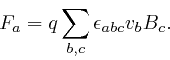
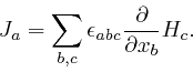
Maxwell interpreted the force on a wire carrying an electric current in the
presence of a magnetic field as being due to a force exerted by the magnetic
field on the moving electric charge carriers in the wire, and defined the
magnetic induction ![]() to be such that, in
Cartesian coordinates, the force
to be such that, in
Cartesian coordinates, the force
![]() on a particle of electric charge
on a particle of electric charge ![]() moving with velocity
moving with velocity ![]() in the
magnetic field
in the
magnetic field ![]() , is:
, is:
Here each index ![]() ,
, ![]() , or
, or ![]() can take values 1, 2, 3, corresponding to the
directions in which the three Cartesian coordinates of spatial position
increase. I explained the meaning of the symbol
can take values 1, 2, 3, corresponding to the
directions in which the three Cartesian coordinates of spatial position
increase. I explained the meaning of the symbol
![]() in the first part of the post,
here.
in the first part of the post,
here.
![]() represents the collection of data that gives the value of the
magnetic field in each coordinate direction at each position in space and each
moment in time, so that if
represents the collection of data that gives the value of the
magnetic field in each coordinate direction at each position in space and each
moment in time, so that if ![]() represents a position in space, the value of
the magnetic field in coordinate direction
represents a position in space, the value of
the magnetic field in coordinate direction ![]() , at position
, at position ![]() , and time
, and time ![]() ,
could be represented as
,
could be represented as ![]() or
or
![]() , for example.
If
, for example.
If ![]() represents the collection of data that gives the particle's position
at each time
represents the collection of data that gives the particle's position
at each time ![]() , then
, then
![]() .
. ![]() represents the collection of data that gives the force on the particle in each
coordinate direction at each moment in time.
represents the collection of data that gives the force on the particle in each
coordinate direction at each moment in time.
The symbol ![]() is an alternative form of the Greek letter
epsilon. The expression
is an alternative form of the Greek letter
epsilon. The expression
![]() is defined to be 1 if the values of
is defined to be 1 if the values of ![]() ,
,
![]() , and
, and ![]() are 1, 2, 3 or 2, 3, 1 or 3, 1, 2;
are 1, 2, 3 or 2, 3, 1 or 3, 1, 2; ![]() if the values of
if the values of ![]() ,
,
![]() , and
, and ![]() are 2, 1, 3 or 3, 2, 1 or 1, 3, 2; and 0 if two or more of the
indexes have the same value. Thus the value of
are 2, 1, 3 or 3, 2, 1 or 1, 3, 2; and 0 if two or more of the
indexes have the same value. Thus the value of
![]() changes by
a factor
changes by
a factor ![]() if any pair of its indexes are swapped. A quantity that
depends on two or more direction indexes is called a tensor, and a quantity
whose value is multiplied by
if any pair of its indexes are swapped. A quantity that
depends on two or more direction indexes is called a tensor, and a quantity
whose value is multiplied by ![]() if two of its indexes of the same type are
swapped is said to be "antisymmetric" in those indexes. Thus
if two of its indexes of the same type are
swapped is said to be "antisymmetric" in those indexes. Thus
![]() is an example of a totally
antisymmetric tensor.
is an example of a totally
antisymmetric tensor.
A quantity that depends on position and time is called a field, and a quantity
that depends on one direction index is called a vector, so the magnetic
induction ![]() is an example of a vector field. From the
above equation, the
unit of the magnetic induction
is an example of a vector field. From the
above equation, the
unit of the magnetic induction ![]() is kilograms per second per coulomb.
is kilograms per second per coulomb.
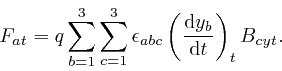
Since no position or time dependence is displayed in the above equation, the
quantities that depend on time are all understood to be evaluated at the same
time, and the equation is understood to be valid for all values of that time.
The magnetic field is understood to be evaluated at the position of the
particle, and the summations over ![]() and
and ![]() are understood to go over all
the values of
are understood to go over all
the values of ![]() and
and ![]() for which the expressions are defined. Thus if we
explicitly displayed all the indexes and the ranges of the summations, the
equation could be written:
for which the expressions are defined. Thus if we
explicitly displayed all the indexes and the ranges of the summations, the
equation could be written:
Maxwell also interpreted the electrostatic force on an electrically charged
particle in the presence of another electrically charged particle as being due
to a force exerted by an electric field produced by the second particle, and
defined the electric field strength ![]() to be such that, in the same notation
as before, the force
to be such that, in the same notation
as before, the force ![]() on a particle of electric charge
on a particle of electric charge ![]() in the electric
field
in the electric
field ![]() , is:
, is:
Thus the unit of the electric field strength ![]() is kilograms metres per
second
is kilograms metres per
second![]() per coulomb, which can also be written as
joules per metre per
coulomb, since a joule, which is the international unit of energy, is one
kilogram metre
per coulomb, which can also be written as
joules per metre per
coulomb, since a joule, which is the international unit of energy, is one
kilogram metre![]() per second
per second![]() . The electric field strength
. The electric field strength ![]() is
another example of a vector field.
is
another example of a vector field.
Electric voltage is the electrical energy in joules per coulomb of electric
charge. Thus if the electrostatic force ![]() can be derived from a potential
energy
can be derived from a potential
energy ![]() by
by
![]() , as in
the example for
which we derived Newton's second law of motion
from de Maupertuis's principle,
then the electric field strength
, as in
the example for
which we derived Newton's second law of motion
from de Maupertuis's principle,
then the electric field strength ![]() is related to
is related to ![]() by
by
![]() . I have written the
potential energy here
as
. I have written the
potential energy here
as ![]() instead of
instead of ![]() , to avoid confusing it with voltage.
, to avoid confusing it with voltage. ![]() is the potential voltage, so the electric field strength is minus the gradient
of the potential voltage, and the unit of electric field strength can also be
expressed as volts per metre.
is the potential voltage, so the electric field strength is minus the gradient
of the potential voltage, and the unit of electric field strength can also be
expressed as volts per metre.
The voltage produced by a voltage source such as a battery can be measured
absolutely by measuring the current that flows and the heat that is produced,
when the terminals of the voltage source are connected through an electrical
resistance. In all currently known electrical conductors at room
temperature, an electric current flowing through the conductor quickly stops
flowing due to frictional effects such as scattering of the moving charge
carriers by the stationary charges in the material, unless the current is
continually driven by a voltage difference between the ends of the conductor,
that produces an electric field along the conductor. The work done by a
voltage source of ![]() volts to move an electric charge of
volts to move an electric charge of ![]() coulombs from
one terminal of the voltage source to the other is
coulombs from
one terminal of the voltage source to the other is ![]() joules, so if a
current of
joules, so if a
current of ![]() amps
amps ![]() coulombs per second is flowing, the work done by the
voltage source per second is
coulombs per second is flowing, the work done by the
voltage source per second is ![]() joules per second
joules per second ![]() watts, since a
watt, which is the international unit of power, is one joule per second.
Thus the voltage
watts, since a
watt, which is the international unit of power, is one joule per second.
Thus the voltage ![]() produced by a voltage source can be measured absolutely
by connecting the terminals of the voltage source by for example a long thin
insulated copper wire that is coiled in a thermally insulated flask of water,
and measuring the electric current
produced by a voltage source can be measured absolutely
by connecting the terminals of the voltage source by for example a long thin
insulated copper wire that is coiled in a thermally insulated flask of water,
and measuring the electric current ![]() and the rate at which the water
temperature rises, since the specific heat capacity of water is known from
measurements by James Joule
to be about 4180 joules per kilogram per degree centigrade.
and the rate at which the water
temperature rises, since the specific heat capacity of water is known from
measurements by James Joule
to be about 4180 joules per kilogram per degree centigrade.
Maxwell summarized Coulomb's law for the electrostatic force between two stationary electric charges by the equation:
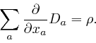
Here ![]() is a vector field called the electric displacement, whose relation to
the electric field strength
is a vector field called the electric displacement, whose relation to
the electric field strength ![]() at a position
at a position ![]() depends on the material
present at
depends on the material
present at ![]() .
.
![]() has the same meaning as
in the first part of the post,
here,
with
has the same meaning as
in the first part of the post,
here,
with ![]() now taken as
now taken as ![]() , and
, and ![]() now taken as
now taken as ![]() .
. ![]() is the
Greek letter rho, and represents the collection of data that gives the amount
of electric charge per unit volume, at each spatial position
is the
Greek letter rho, and represents the collection of data that gives the amount
of electric charge per unit volume, at each spatial position ![]() and time
and time ![]() .
It is called the electric charge density. For each position
.
It is called the electric charge density. For each position ![]() and time
and time
![]() , it is defined to be the amount of
electric charge inside a small volume
, it is defined to be the amount of
electric charge inside a small volume
![]() centred at
centred at ![]() , divided by
, divided by ![]() , where the ratio is
taken in the limit that
, where the ratio is
taken in the limit that ![]() tends to 0. A field that does not
depend on any direction indexes is called a scalar field, so
tends to 0. A field that does not
depend on any direction indexes is called a scalar field, so ![]() is an
example of a scalar field. The units of
is an
example of a scalar field. The units of ![]() are coulombs per metre
are coulombs per metre![]() ,
so the units of
,
so the units of ![]() are coulombs per metre
are coulombs per metre![]() .
.
In most materials the electric displacement ![]() and the electric field
strength
and the electric field
strength ![]() are related by:
are related by:
where ![]() is a number called the permittivity
of the material. Although the same symbol is used for the permittivity and the
antisymmetric tensor
is a number called the permittivity
of the material. Although the same symbol is used for the permittivity and the
antisymmetric tensor
![]() , I will always show the indices on
, I will always show the indices on
![]() , so that it can't be mistaken for the permittivity.
, so that it can't be mistaken for the permittivity.
To check that the
above equation summarizing Coulomb's law leads to the
inverse square law for the electrostatic force between stationary point-like
charges as measured by Coulomb, we'll calculate the electric field produced by
a small electrically charged sphere. We'll choose the zero of each of the
three Cartesian coordinates to be at the centre of the sphere, and represent
the radius of the sphere by ![]() . The electric charge per unit volume,
. The electric charge per unit volume,
![]() , might depend on position in the sphere,
for example the charge might
be concentrated in a thin layer just inside the surface of the sphere. We'll
assume that
, might depend on position in the sphere,
for example the charge might
be concentrated in a thin layer just inside the surface of the sphere. We'll
assume that ![]() , the value of
, the value of ![]() at position
at position ![]() , does not depend on
the direction from
, does not depend on
the direction from ![]() to the centre of the sphere, although it might depend
on the distance
to the centre of the sphere, although it might depend
on the distance
![]() from
from ![]() to the centre of
the sphere. The electric displacement
to the centre of
the sphere. The electric displacement ![]() at position
at position ![]() will be directed
along the straight line from
will be directed
along the straight line from ![]() to the centre of the sphere, so
to the centre of the sphere, so ![]() for
for ![]() , where
, where ![]() is a quantity that depends on
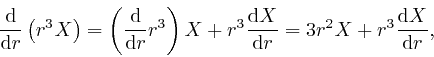
is a quantity that depends on ![]() . From
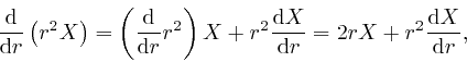
Leibniz's rule for the rate of change of a product, which we obtained in
the first part of the post,
here,
we have:
. From
Leibniz's rule for the rate of change of a product, which we obtained in
the first part of the post,
here,
we have:
And since ![]() only depends on
only depends on ![]() through the dependence of
through the dependence of ![]() on
on ![]() , we
have:
, we
have:
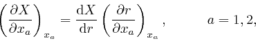
The values of the components of ![]() other than
other than ![]() are fixed throughout this
formula, so their values don't need to be displayed. From this formula and
the previous one:
are fixed throughout this
formula, so their values don't need to be displayed. From this formula and
the previous one:
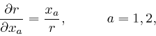
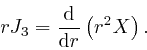
Leibniz's rule for the rate of change of a product also gives us:
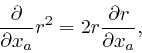
and since
![]() , it also gives us:
, it also gives us:
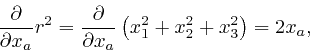
since, for example,
![]() , while
, while
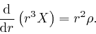
![]() . Thus
. Thus

so from the previous formula,
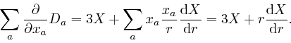
Thus from Maxwell's equation summarizing Coulomb's law, above:
From Leibniz's rule for the rate of change of a product, we have:
where the final equality follows from the result
![]() we obtained in the second part of the
post,
here,
with
we obtained in the second part of the
post,
here,
with ![]() taken as 3 and
taken as 3 and ![]() taken as
taken as
![]() . Thus after multiplying the previous equation by
. Thus after multiplying the previous equation by ![]() , it can be
written:
, it can be
written:
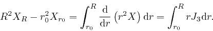
So from the result we found in the first part of the post,
here,
that the integral of the rate of change of
a quantity is equal to the net change of that quantity, we find that for any
two particular values ![]() and
and ![]() of
of ![]() :
:
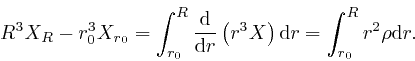
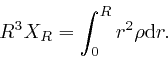
The expression
 is the total electric
charge in the region between distances
is the total electric
charge in the region between distances ![]() and
and ![]() from the centre of the
sphere, divided by the surface area of a sphere of radius 1, which I'll
represent by
from the centre of the
sphere, divided by the surface area of a sphere of radius 1, which I'll
represent by ![]() . For the surface area of a sphere of radius
. For the surface area of a sphere of radius ![]() is
is ![]() ,
since if we use angular coordinates such as latitude and longitude to specify
position on the surface of the sphere, the distance moved as a result of a
change of an angular coordinate is proportional to
,
since if we use angular coordinates such as latitude and longitude to specify
position on the surface of the sphere, the distance moved as a result of a
change of an angular coordinate is proportional to ![]() . Thus the
contribution to the integral
from the
interval from
. Thus the
contribution to the integral
from the
interval from ![]() to
to
![]() is aproximately
is aproximately ![]() times
the total electric charge in the spherical shell between distances
times
the total electric charge in the spherical shell between distances ![]() and
and
![]() from
from
![]() , since the volume of this shell
is approximately
, since the volume of this shell
is approximately
![]() , and the errors of these two
approximations tend to 0 more rapidly than in proportion to
, and the errors of these two
approximations tend to 0 more rapidly than in proportion to ![]() as
as
![]() tends to 0.
tends to 0.
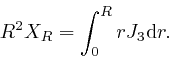
Let's now assume that ![]() is finite throughout the sphere, and depends
smoothly on
is finite throughout the sphere, and depends
smoothly on ![]() as
as ![]() tends to 0. Then
tends to 0. Then ![]() is finite as
is finite as ![]() tends
to 0, so:
tends
to 0, so:
Thus for ![]() greater than the radius
greater than the radius ![]() of the charged sphere, we have:
of the charged sphere, we have:
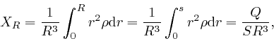
where ![]() is the total electric charge of the sphere. Thus if
is the total electric charge of the sphere. Thus if ![]() is outside
the sphere, then the electric displacement
is outside
the sphere, then the electric displacement ![]() at
at ![]() is given by:
is given by:
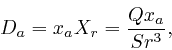
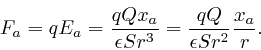
for ![]() . Thus the electric field strength
. Thus the electric field strength ![]() in the region
outside the sphere is given by:
in the region
outside the sphere is given by:
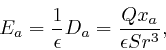
where ![]() is the permittivity of the material
in the region outside the
sphere. So the force
is the permittivity of the material
in the region outside the
sphere. So the force ![]() on a particle of electric charge
on a particle of electric charge ![]() at position
at position
![]() outside the sphere is given by:
outside the sphere is given by:
This is in agreement with Coulomb's law, since ![]() is a vector of
length 1, that points along the line from the centre of the sphere to
is a vector of
length 1, that points along the line from the centre of the sphere to ![]() . The force is repulsive if
. The force is repulsive if ![]() and
and ![]() have the same sign, and attractive if
they have opposite signs.
have the same sign, and attractive if
they have opposite signs.
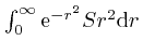
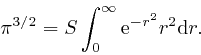
We'll calculate the surface area ![]() of a sphere of radius 1 by using the
result we found in the second part of the post,
here, that
of a sphere of radius 1 by using the
result we found in the second part of the post,
here, that
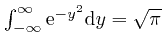 . We have:
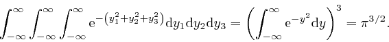
We can also think of ![]() ,
, ![]() , and
, and ![]() as the Cartesian coordinates of a
point in
3-dimensional Euclidean space.
The distance
as the Cartesian coordinates of a
point in
3-dimensional Euclidean space.
The distance ![]() from the point
from the point
![]() to the point
to the point
![]() is then
is then
![]() . So from the discussion
above,
with
. So from the discussion
above,
with
![]() taken as
taken as
![]() , the above triple integral is equal to
, the above triple integral is equal to
 , so we have:
The value of the expression
![]() is unaltered if we
replace
is unaltered if we
replace ![]() by
by ![]() , so we also have:
, so we also have:
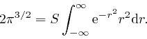
So from the result we found in the second part of the post, here:
Thus the force ![]() on a particle of electric charge
on a particle of electric charge ![]() at position
at position ![]() outside the sphere is given by:
outside the sphere is given by:
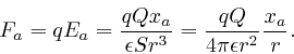
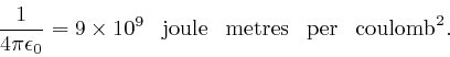
The permittivity of the vacuum is denoted by ![]() . The expression
. The expression
![]() is the number that determines the overall
strength of the electrostatic force between two stationary charges, so it
plays the same role for the electrostatic force as Newton's constant
is the number that determines the overall
strength of the electrostatic force between two stationary charges, so it
plays the same role for the electrostatic force as Newton's constant ![]() plays
for the gravitational force.
plays
for the gravitational force.
The value of the permittivity, ![]() , whose unit is joule metres per
coulomb
, whose unit is joule metres per
coulomb![]() , or equivalently kilogram metre
, or equivalently kilogram metre![]() per second
per second![]() per
coulomb
per
coulomb![]() , can be measured for a particular electrical insulator by placing
a sample of the insulator between the plates of a parallel plate capacitor,
which consists of two large parallel conducting plates separated by a thin
layer of insulator, then connecting a known voltage source across the plates
of the capacitor, and measuring the time integral of the resulting current
that flows along the wires from the voltage source to the capacitor, until the
current stops flowing. The current is
, can be measured for a particular electrical insulator by placing
a sample of the insulator between the plates of a parallel plate capacitor,
which consists of two large parallel conducting plates separated by a thin
layer of insulator, then connecting a known voltage source across the plates
of the capacitor, and measuring the time integral of the resulting current
that flows along the wires from the voltage source to the capacitor, until the
current stops flowing. The current is ![]() the rate of change of the charge
on a plate of the capacitor, so since the integral of the rate of change is
the net change, as we found in the first part of the post,
here, the time integral of the current is
the rate of change of the charge
on a plate of the capacitor, so since the integral of the rate of change is
the net change, as we found in the first part of the post,
here, the time integral of the current is ![]() the total electric charge that ends up on a plate of the capacitor.
the total electric charge that ends up on a plate of the capacitor.
Once the current has stopped flowing, the voltage no longer changes along the
wires from the terminals of the voltage source to the plates of the capacitor,
so the entire voltage of the voltage source ends up between the plates of the
capacitor. If the lengths of the sides of the capacitor plates are much
larger than the distance between the plates, and the 1 and 2 coordinate
directions are in the plane of the plates, then the electric field strength
between the plates is
![]() , where
, where ![]() is the voltage of the
voltage source, and
is the voltage of the
voltage source, and ![]() is the distance between the plates.
is the distance between the plates.
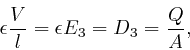
If the electric charge on a plate of the capacitor is ![]() and is uniformly
distributed over the capacitor plate, and the area of each capacitor plate is
and is uniformly
distributed over the capacitor plate, and the area of each capacitor plate is
![]() , then by integrating Maxwell's equation
, then by integrating Maxwell's equation
![]() across the thickness of a capacitor plate and noting that the electric
field is 0 outside the plates, we find:
across the thickness of a capacitor plate and noting that the electric
field is 0 outside the plates, we find:
since the integral of
![]() across the thickness
of a capacitor plate is equal to the difference of
across the thickness
of a capacitor plate is equal to the difference of ![]() between the inner and
outer faces of that capacitor plate, by the result we found in the first part of
the post,
here, that the
integral of the rate of change of a quantity is equal to the net change of
that quantity; and the integral of the electric charge per unit volume,
between the inner and
outer faces of that capacitor plate, by the result we found in the first part of
the post,
here, that the
integral of the rate of change of a quantity is equal to the net change of
that quantity; and the integral of the electric charge per unit volume,
![]() , across the thickness of a capacitor plate is equal to the electric
charge per unit area,
, across the thickness of a capacitor plate is equal to the electric
charge per unit area, ![]() , on the capacitor plate.
, on the capacitor plate.
Thus since ![]() ,
, ![]() ,
, ![]() , and
, and ![]() are all known, the value of
are all known, the value of ![]() for
the electrical insulator between the capacitor plates is determined. From
measurements of this type with a vacuum between the capacitor plates, the
permittivity
for
the electrical insulator between the capacitor plates is determined. From
measurements of this type with a vacuum between the capacitor plates, the
permittivity ![]() of a vacuum is found to be such that:
of a vacuum is found to be such that:
Maxwell summarized Ampère's law for the force between two parallel electric currents, as above, by the equation:
Here ![]() is a vector field called the electric current density. For each
position
is a vector field called the electric current density. For each
position ![]() , time
, time ![]() , and value 1, 2, or 3 of the coordinate index
, and value 1, 2, or 3 of the coordinate index ![]() , it
is defined to be the net amount of electric charge that passes in the positive
, it
is defined to be the net amount of electric charge that passes in the positive
![]() direction through a small area
direction through a small area ![]() perpendicular to the
perpendicular to the ![]() direction in a small time
direction in a small time ![]() , divided by
, divided by
![]() , where the ratio is taken in the limit that
, where the ratio is taken in the limit that ![]() and
and ![]() tend to 0. The units of
tend to 0. The units of ![]() are amps per metre
are amps per metre![]() .
.
![]() is the totally antisymmetric tensor I defined
above.
is the totally antisymmetric tensor I defined
above.
![]() is a vector field
called the magnetic field strengh, whose relation to the magnetic induction
is a vector field
called the magnetic field strengh, whose relation to the magnetic induction
![]() at a position
at a position ![]() depends on the material present at
depends on the material present at ![]() . The units of
. The units of
![]() are amps per metre.
are amps per metre.
![]() has the same meaning
as in the first part of the post,
here,
with
has the same meaning
as in the first part of the post,
here,
with ![]() now taken as
now taken as ![]() , and
, and ![]() now taken as
now taken as ![]() .
.
In most non-magnetized materials the magnetic induction ![]() and the magnetic
field strength
and the magnetic
field strength ![]() are related by:
are related by:
where ![]() , which is the Greek letter mu, is a number called the permeability
of the material. Its unit is kilogram metres per coulomb
, which is the Greek letter mu, is a number called the permeability
of the material. Its unit is kilogram metres per coulomb![]() . The
permeability of the vacuum is denoted by
. The
permeability of the vacuum is denoted by ![]() . Its value is fixed by the
definition of the amp, as
above.
. Its value is fixed by the
definition of the amp, as
above.
To check that the
above
equation summarizing Ampère's law leads to a force
between two long straight parallel wires carrying electric currents, whose
strength is inversely proportional to the distance between the wires as
measured by Ampère, and to calculate the value of ![]() implied by the
definition of the amp, as
above,
we'll calculate the magnetic field produced by an
infinitely long straight wire that is carrying an electric current. We'll
choose the wire to be along the 3 direction, and the zero of the 1 and 2
Cartesian coordinates to be at the centre of the wire, and represent the
radius of the wire by
implied by the
definition of the amp, as
above,
we'll calculate the magnetic field produced by an
infinitely long straight wire that is carrying an electric current. We'll
choose the wire to be along the 3 direction, and the zero of the 1 and 2
Cartesian coordinates to be at the centre of the wire, and represent the
radius of the wire by ![]() . We'll assume that
. We'll assume that ![]() , the electric current
density in the direction along the wire at position
, the electric current
density in the direction along the wire at position ![]() , does not depend on
, does not depend on
![]() or the direction from
or the direction from ![]() to the centre of the wire, although it might
depend on the distance
to the centre of the wire, although it might
depend on the distance
![]() from
from ![]() to the centre of
the wire.
to the centre of
the wire.
From its definition
above,
the antisymmetric tensor
![]() is 0 if
any two of its indexes are equal, so in particular,
is 0 if
any two of its indexes are equal, so in particular,
![]() is 0
for all values of the index
is 0
for all values of the index ![]() . Thus Maxwell's equation summarizing
Ampère's law, as
above,
does not relate
. Thus Maxwell's equation summarizing
Ampère's law, as
above,
does not relate ![]() to
to ![]() , so we'll assume
, so we'll assume ![]() is 0.
is 0.
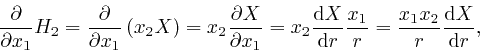
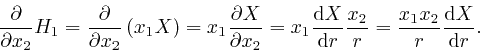
Now let's suppose that the magnetic field strength ![]() at position
at position ![]() is
directed along the straight line perpendicular to the wire from
is
directed along the straight line perpendicular to the wire from ![]() to the
centre of the wire, so
to the
centre of the wire, so ![]() for
for ![]() , where
, where ![]() is a quantity
that depends on
is a quantity
that depends on ![]() . Then in the same way as
above,
we find:
. Then in the same way as
above,
we find:
and also in the same way as above, we find:
so:
From Leibniz's rule for the rate of change of a product, which we obtained in the first part of the post, here, we have:
Thus:
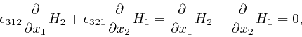
so Maxwell's equation summarizing Ampère's law, as
above,
does not relate
![]() to this form of
to this form of ![]() , so we'll also assume that this form of
, so we'll also assume that this form of ![]() is 0.
is 0.
The final possibility is that the magnetic field strength ![]() at position
at position ![]() is perpendicular to the plane defined by
is perpendicular to the plane defined by ![]() and the wire carrying the
current. Then
and the wire carrying the
current. Then ![]() , and from the diagram in the first
part of the post,
here,
interpreted as the
two-dimensional plane through
, and from the diagram in the first
part of the post,
here,
interpreted as the
two-dimensional plane through ![]() and perpendicular to the wire, if
and perpendicular to the wire, if
![]() and
and
![]() , then the direction of
, then the direction of ![]() is along
is along
![]() , so
, so ![]() ,
, ![]() , where
, where ![]() is a quantity that
depends on
is a quantity that
depends on ![]() . Then from Leibniz's rule for the rate of change of a
product, which we obtained in the first part of the post,
here, and the formula
above for
. Then from Leibniz's rule for the rate of change of a
product, which we obtained in the first part of the post,
here, and the formula
above for
![]() , we have:
, we have:


Thus from Maxwell's equation summarizing Ampère's law, as above:

From Leibniz's rule for the rate of change of a product, we have:
where the final equality follows from the result
![]() we obtained in the second part of
the post,
here,
with
we obtained in the second part of
the post,
here,
with ![]() taken as 2 and
taken as 2 and ![]() taken as
taken as
![]() . Thus after multiplying the previous equation by
. Thus after multiplying the previous equation by ![]() , it can be written:
, it can be written:
So from the result we found in the first part of the post,
here,
that the integral of the rate of change of
a quantity is equal to the net change of that quantity, we find that for any
two particular values ![]() and
and ![]() of
of ![]() :
:
The expression
 is
is
![]() times the
total electric charge per unit time passing through the region between
distances
times the
total electric charge per unit time passing through the region between
distances ![]() and
and ![]() from the centre of the wire, in any cross-section of
the wire. For the circumference of a circle of radius
from the centre of the wire, in any cross-section of
the wire. For the circumference of a circle of radius ![]() is
is ![]() , so
the contribution to the integral
from the
interval from
, so
the contribution to the integral
from the
interval from ![]() to
to
![]() is aproximately
is aproximately
![]() times the total electric charge per unit time passing through the region
between distances
times the total electric charge per unit time passing through the region
between distances ![]() and
and
![]() from the centre of the wire, in
any cross-section of the wire, since the area of this shell is approximately
from the centre of the wire, in
any cross-section of the wire, since the area of this shell is approximately
![]() , and the errors of these two approximations tend to 0
more rapidly than in proportion to
, and the errors of these two approximations tend to 0
more rapidly than in proportion to ![]() as
as ![]() tends to
0.
tends to
0.
Let's now assume that ![]() is finite throughout the cross-section of the
wire, and depends smoothly on
is finite throughout the cross-section of the
wire, and depends smoothly on ![]() as
as ![]() tends to 0. Then
tends to 0. Then ![]() is
finite as
is
finite as ![]() tends to 0, so:
tends to 0, so:
Thus for ![]() greater than the radius
greater than the radius ![]() of the wire, we have:
of the wire, we have:
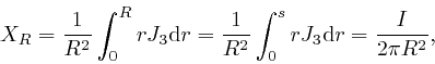
where ![]() is the total electric current carried by the wire. Thus if
is the total electric current carried by the wire. Thus if ![]() is
outside the wire, then the magnetic field strength
is
outside the wire, then the magnetic field strength ![]() at
at ![]() is given by:
is given by:
Thus the magnetic induction ![]() in the region outside the wire is given by:
in the region outside the wire is given by:
where ![]() is the permeability of the material in the region outside the
wire. This is perpendicular to the plane defined by the point and the wire,
and its magnitude is proportional to the current in the wire, and inversely
proportional to the distance of the point from the wire, in agreement with the
measurements of Biot and Savart as
above,
since
is the permeability of the material in the region outside the
wire. This is perpendicular to the plane defined by the point and the wire,
and its magnitude is proportional to the current in the wire, and inversely
proportional to the distance of the point from the wire, in agreement with the
measurements of Biot and Savart as
above,
since
![]() is a vector of length 1.
is a vector of length 1.
Let's now suppose there is a second infinitely long straight wire parallel to
the first, such that the 1 and 2 Cartesian coordinates of the centre of the
second wire are
![]() , and the total electric current
carried by the second wire is
, and the total electric current
carried by the second wire is
![]() .
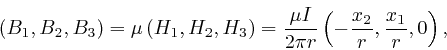
From Maxwell's equation
above, and the definition of the antisymmetric
tensor
.
From Maxwell's equation
above, and the definition of the antisymmetric
tensor
![]() as
above, the force
as
above, the force ![]() on a particle of electric
charge
on a particle of electric
charge ![]() moving with velocity
moving with velocity
![]() along the
second wire, in the presence of the magnetic field
along the
second wire, in the presence of the magnetic field ![]() produced by the first
wire, as above, is given by:
produced by the first
wire, as above, is given by:
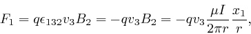
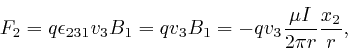
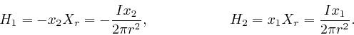
The interaction between this moving charge and the other particles in the
second wire prevents this moving charge from accelerating sideways out of the
second wire, so the above force is a contribution to the force on the second
wire, that results from the magnetic field ![]() produced by the current in the
first wire. If there are
produced by the current in the
first wire. If there are ![]() particles of electric charge
particles of electric charge ![]() and velocity
and velocity
![]() per unit length of the second wire, then their
contribution to the force per unit length on the second wire is:
per unit length of the second wire, then their
contribution to the force per unit length on the second wire is:
The average number of these particles that pass through any cross-section of
the second wire per unit time is ![]() , so their contribution to the electric
current carried by the second wire is
, so their contribution to the electric
current carried by the second wire is ![]() . Thus the contribution of
these particles to the force per unit length on the second wire is
. Thus the contribution of
these particles to the force per unit length on the second wire is
![]() times
their contribution to the electric current carried by the second wire. So by
adding up the contributions from charged particles of all relevant values of
times
their contribution to the electric current carried by the second wire. So by
adding up the contributions from charged particles of all relevant values of
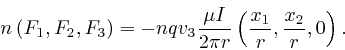
![]() and
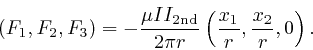
and ![]() , we find that the total force
, we find that the total force ![]() per unit length on the second
wire that results from the current
per unit length on the second
wire that results from the current ![]() carried by the first wire and the
current
carried by the first wire and the
current
![]() carried by the second
wire is given by:
carried by the second
wire is given by:
The direction of this force is towards the first wire if ![]() and
and
![]() have the same sign and away
from the first wire if
have the same sign and away
from the first wire if ![]() and
and
![]() have opposite sign, and the strength of this force is proportional to the
product of the currents, and inversely proportional to the distance between
the wires, so this force is in agreement with Ampère's law, as
above.
And
from the definition of the amp, as
above,
we find that the permeability
have opposite sign, and the strength of this force is proportional to the
product of the currents, and inversely proportional to the distance between
the wires, so this force is in agreement with Ampère's law, as
above.
And
from the definition of the amp, as
above,
we find that the permeability
![]() of a vacuum is by definition given by:
of a vacuum is by definition given by:
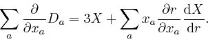
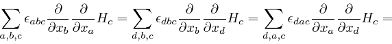
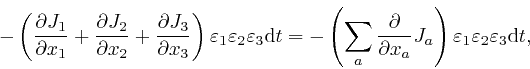
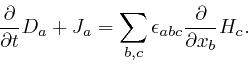
Maxwell noticed that his equation summarizing Ampère's law, as
above,
leads to
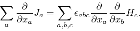
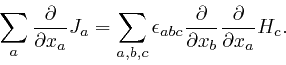
a contradiction. For by applying
![]() to both
sides of that equation, and summing over
to both
sides of that equation, and summing over ![]() , we obtain:
, we obtain:
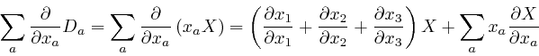
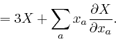
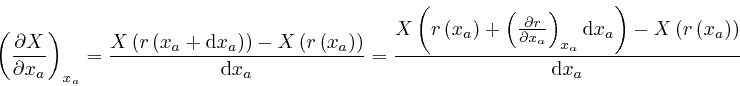
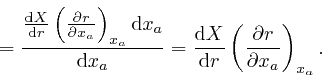
For a quantity ![]() that depends smoothly on a number of quantities
that depends smoothly on a number of quantities ![]() that
can vary continuously, where
that
can vary continuously, where ![]() represents the collection of those
quantities, and indexes such as
represents the collection of those
quantities, and indexes such as ![]() or
or ![]() distinguish the quantities in the
collection, we have:
distinguish the quantities in the
collection, we have:
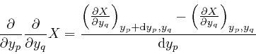
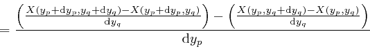

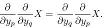
The expression in the third line here is equal to the expression we obtain
from it by swapping the indexes ![]() and
and ![]() , so we have:
, so we have:
So if the magnetic field strength ![]() depends smoothly on position, we also
have:
depends smoothly on position, we also
have:
The value of the right-hand side of this formula does not depend on the
particular letters ![]() ,
, ![]() , and
, and ![]() used for the indexes that are summed
over. Thus if the letter
used for the indexes that are summed
over. Thus if the letter ![]() , used as an index, is also understood to have
the possible values 1, 2, or 3, we have:
, used as an index, is also understood to have
the possible values 1, 2, or 3, we have:
At each of the first three steps in the above formula, one of the indexes
summed over in the previous version of the expression is rewritten as a
different letter that is understood to take the same possible values, 1, 2, or
3, and which does not otherwise occur in the expression. At the first step,
the index ![]() is rewritten as
is rewritten as ![]() , then at the second step, the index
, then at the second step, the index ![]() is
rewritten as
is
rewritten as ![]() , and at the third step, the index
, and at the third step, the index ![]() is rewritten as
is rewritten as ![]() . An index that occurs in an expression, but is summed over the range of its
possible values, so that the full expression, including the
. An index that occurs in an expression, but is summed over the range of its
possible values, so that the full expression, including the ![]() , does not
depend on the value of that index, is called a "dummy index".
, does not
depend on the value of that index, is called a "dummy index".
The fourth step in the above formula used the definition of the antisymmetric
tensor
![]() , as
above,
which implies that its value is
multiplied by
, as
above,
which implies that its value is
multiplied by ![]() if two of its indexes are swapped, so that
if two of its indexes are swapped, so that
![]() . The fifth step used the original formula for
. The fifth step used the original formula for
![]() , as
above,
together with the fact
that the order of the indexes under the
, as
above,
together with the fact
that the order of the indexes under the ![]() in the right-hand side doesn't
matter, since each of the indexes is simply summed over the values 1, 2, and
3.
in the right-hand side doesn't
matter, since each of the indexes is simply summed over the values 1, 2, and
3.
Thus from the second formula for
![]() ,
as
above,
we have:
,
as
above,
we have:
Hence:
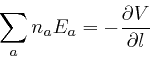
Let's now consider the rate of change with time of the total electric charge
in a tiny box-shaped region centred at a position ![]() , such that the edges of
the box are aligned with the coordinate directions, and have lengths
, such that the edges of
the box are aligned with the coordinate directions, and have lengths
![]() ,
, ![]() , and
, and ![]() . From the definition
above
of the electric current density
. From the definition
above
of the electric current density ![]() , the net amount of electric charge
that flows into the box through the face of the box perpendicular to the 1
direction and centred at
, the net amount of electric charge
that flows into the box through the face of the box perpendicular to the 1
direction and centred at
![]() , during a small time
, during a small time ![]() , is approximately
, is approximately
![]() , and the net amount of electric charge that flows out of the box
through the face of the box perpendicular to the 1 direction and centred at
, and the net amount of electric charge that flows out of the box
through the face of the box perpendicular to the 1 direction and centred at
![]() , during the same
small time
, during the same
small time ![]() , is approximately
, is approximately
![]() , and
the errors of these approximations tend to 0 more rapidly than in proportion
to
, and
the errors of these approximations tend to 0 more rapidly than in proportion
to
![]() , as
, as ![]() ,
,
![]() , and
, and ![]() tend to 0. And from the result we
obtained in the first part of the post,
here,
with
tend to 0. And from the result we
obtained in the first part of the post,
here,
with
![]() taken as
taken as ![]() and
and ![]() taken as
taken as
![]() , we have:
, we have:
where the error of the above approximations tends to 0 more rapidly than in
proportion to ![]() , as
, as ![]() tends to 0. Thus the net
amount of electric charge that flows into the box through the faces of the box
perpendicular to the 1 direction, during a small time
tends to 0. Thus the net
amount of electric charge that flows into the box through the faces of the box
perpendicular to the 1 direction, during a small time ![]() , is
approximately:
, is
approximately:

where the error of this approximation tends to 0 more rapidly than in
proportion to
![]() , as
, as
![]() ,
, ![]() ,
, ![]() , and
, and ![]() tend to
0. So from the corresponding results for the net amount of electric charge
that flows into the box through the faces of the box perpendicular to the 2
and 3 directions, during the same small time
tend to
0. So from the corresponding results for the net amount of electric charge
that flows into the box through the faces of the box perpendicular to the 2
and 3 directions, during the same small time ![]() , we find that the
net amount of electric charge that flows into the box through all the faces of
the box, during the small time
, we find that the
net amount of electric charge that flows into the box through all the faces of
the box, during the small time ![]() , is approximately:
, is approximately:
where the error of this approximation tends to 0 more rapidly than in
proportion to
![]() , as
, as
![]() ,
, ![]() ,
, ![]() , and
, and ![]() tend to
0.
tend to
0.
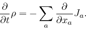
There's no evidence that electric charge can vanish into nothing or appear
from nothing, so the net amount of electric charge that flows into the box
through all the faces of the box, during the small time ![]() , must
be equal to the net increase of the total electric charge in the box, during
the small time
, must
be equal to the net increase of the total electric charge in the box, during
the small time ![]() , which from the definition of the electric
charge density
, which from the definition of the electric
charge density ![]() , as
above,
is approximately:
, as
above,
is approximately:
where the error of this approximation tends to 0 more rapidly than in
proportion to
![]() , as
, as
![]() ,
, ![]() ,
, ![]() , and
, and ![]() tend to
0. Thus we must have:
tend to
0. Thus we must have:
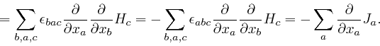
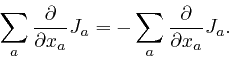
But we found
above
that Maxwell's equation summarizing Ampère's law, as
above,
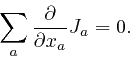
leads instead to
![]() . This
equation is false whenever there is a build-up of electric charge in a region,
as, for example, on the plates of a parallel plate capacitor, in the method of
measuring the permittivity
. This
equation is false whenever there is a build-up of electric charge in a region,
as, for example, on the plates of a parallel plate capacitor, in the method of
measuring the permittivity ![]() of an electrical insulator, that I
described above. Maxwell realized that the resolution of this paradox is
that there must be an additional term
of an electrical insulator, that I
described above. Maxwell realized that the resolution of this paradox is
that there must be an additional term
![]() in the
left-hand side of his equation summarizing Ampère's law, where
in the
left-hand side of his equation summarizing Ampère's law, where ![]() is the
electric displacement vector field, so that the corrected form of his equation
summarizing Ampère's law is:
is the
electric displacement vector field, so that the corrected form of his equation
summarizing Ampère's law is:
This equation still correctly reproduces Ampère's law and the magnetic field
produced by an electric current flowing in a long straight wire as measured by
Biot and Savart, as I described
above,
because the experiments of Ampère and
Biot and Savart were carried out in steady state conditions, where nothing
changed with time, so the new term in the left-hand side gave 0. However if
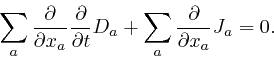
we apply
![]() to both sides of this corrected
equation, and sum over
to both sides of this corrected
equation, and sum over ![]() , which is what led to the paradox for the original
equation, we now find:
, which is what led to the paradox for the original
equation, we now find:
So if the electric displacement ![]() depends smoothly on position, so that
depends smoothly on position, so that
![]() , by the result
we found
above,
we find:
, by the result
we found
above,
we find:
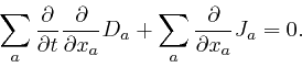
Combining this with Maxwell's equations summarizing Coulomb's law, as above, it gives:
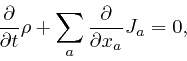
which is now in agreement with the formula expressing the conservation of electric charge, as above.
Michael Faraday
discovered in 1831 that if an electrically insulated wire is
arranged so that somewhere along its length it forms a loop, and the magnetic
induction field ![]() inside the loop and perpendicular to the plane of the loop
is changed, for example by switching on a current in a separate coil of wire
in a suitable position near the loop, then a voltage
inside the loop and perpendicular to the plane of the loop
is changed, for example by switching on a current in a separate coil of wire
in a suitable position near the loop, then a voltage ![]() is temporarily
generated along the wire while the magnetic induction field
is temporarily
generated along the wire while the magnetic induction field ![]() is changing,
such that if the directions of the 1 and 2 Cartesian coordinates are in the
plane of the loop, and the value of
is changing,
such that if the directions of the 1 and 2 Cartesian coordinates are in the
plane of the loop, and the value of ![]() in the region enclosed by the loop
in the plane of the loop depends on time but not on position within that
region, then:
in the region enclosed by the loop
in the plane of the loop depends on time but not on position within that
region, then:

where ![]() is the area enclosed by the loop, and the sign depends on the
direction along the wire in which the voltage is measured. The sign of the
voltage is such that if a current flows along the wire in consequence of the
voltage, then the magnetic field
is the area enclosed by the loop, and the sign depends on the
direction along the wire in which the voltage is measured. The sign of the
voltage is such that if a current flows along the wire in consequence of the
voltage, then the magnetic field
![]() produced by that current, as
above,
is such that
produced by that current, as
above,
is such that
![]() in the region enclosed by the loop in the plane of the loop has the
opposite sign to
in the region enclosed by the loop in the plane of the loop has the
opposite sign to
![]() .
.
Maxwell assumed that the electric field strength ![]() that corresponds to the
voltage
that corresponds to the
voltage ![]() is produced by the changing magnetic induction field
is produced by the changing magnetic induction field ![]() even when
there is no wire present to detect
even when
there is no wire present to detect ![]() in a convenient way. To discover the
consequences of this assumption, it is helpful to know about the relation
between the electric field strength
in a convenient way. To discover the
consequences of this assumption, it is helpful to know about the relation
between the electric field strength ![]() and the rate of change of voltage with
distance in a particular direction.
and the rate of change of voltage with
distance in a particular direction.
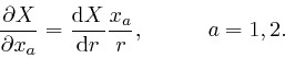
For any vector ![]() , and any vector
, and any vector ![]() of length 1, the expression
of length 1, the expression
![]() is called the component of
is called the component of ![]() in the direction
in the direction ![]() . To relate this to
the magnitude
. To relate this to
the magnitude
![]() of
of ![]() , which is
, which is
![]() by
Pythagoras, and the angle
by
Pythagoras, and the angle ![]() between the directions of
between the directions of ![]() and
and ![]() , we
observe that
, we
observe that
![]() is a vector of length 1, and if we
consider
is a vector of length 1, and if we
consider ![]() and
and
![]() as representing the Cartesian
coordinates of two points in the 3-dimensional generalization of Euclidean
geometry, as in the first part of this post,
here,
then by Pythagoras, the distance between those points is:
as representing the Cartesian
coordinates of two points in the 3-dimensional generalization of Euclidean
geometry, as in the first part of this post,
here,
then by Pythagoras, the distance between those points is:
If ![]() does not point either in the same direction as
does not point either in the same direction as ![]() or the opposite
direction to
or the opposite
direction to ![]() , so that
, so that ![]() is not equal to
is not equal to
![]() , then the directions of
, then the directions of ![]() and
and ![]() define a 2-dimensional plane,
and we can choose Cartesian coordinates in that 2-dimensional plane as in
the first part of the post,
here,
such that the coordinates of
define a 2-dimensional plane,
and we can choose Cartesian coordinates in that 2-dimensional plane as in
the first part of the post,
here,
such that the coordinates of ![]() are
are
![]() , and the
coordinates of
, and the
coordinates of
![]() are
are
![]() . So by
Pythagoras, the distance between the points they define is:
. So by
Pythagoras, the distance between the points they define is:
This is equal to the previous expression, so we have:
This formula is also true when
![]() , so
, so
![]() . If
. If ![]() is along the
is along the ![]() coordinate direction, this formula shows that
coordinate direction, this formula shows that
![]() , where
, where ![]() is the angle between
the direction of
is the angle between
the direction of ![]() and the
and the ![]() coordinate direction. Thus for any vector
coordinate direction. Thus for any vector
![]() of length 1,
of length 1,
![]() is equal to the value that the coordinate of
is equal to the value that the coordinate of
![]() in the direction
in the direction ![]() would have, if
would have, if ![]() was one of the coordinate
directions of Cartesian coordinates.
was one of the coordinate
directions of Cartesian coordinates.
If the electric field strength ![]() can be derived from a voltage field
can be derived from a voltage field ![]() , so
that
, so
that
![]() as
above,
then at each point
along the electrically insulated wire, we have:
as
above,
then at each point
along the electrically insulated wire, we have:
where ![]() is the distance along the wire from that point to a fixed end of the
wire, and
is the distance along the wire from that point to a fixed end of the
wire, and ![]() is a vector of length 1 whose direction is along the wire in
the direction of increasing
is a vector of length 1 whose direction is along the wire in
the direction of increasing ![]() . The first equality here is the component of
the equation
. The first equality here is the component of
the equation
![]() in the direction along
the wire. The component of
in the direction along
the wire. The component of
![]() in any
direction is the rate of change of
in any
direction is the rate of change of ![]() with distance in that direction, so the
component of
with distance in that direction, so the
component of
![]() in the direction along the wire
is the rate of change of
in the direction along the wire
is the rate of change of ![]() with distance along the wire, which is the second
equality.
with distance along the wire, which is the second
equality.
The movable electrically charged particles in the wire are channelled by the
electrical insulation of the wire so that their net motion can only be along
the wire, and only the component of the electric field strength along the wire
can affect their net motion. Their motion along the wire due to the force
![]() is determined by a voltage
is determined by a voltage ![]() defined
along the wire such that
defined
along the wire such that
as in the previous formula, even if the voltage ![]() defined along the wire
does not correspond to a voltage field in the region outside the wire.
defined along the wire
does not correspond to a voltage field in the region outside the wire.
Let's consider Faraday's result, as
above,
for a very small rectangular loop centred at
![]() , such that the edges of
the loop are in the 1 and 2
Cartesian coordinate directions and have lengths
, such that the edges of
the loop are in the 1 and 2
Cartesian coordinate directions and have lengths ![]() and
and
![]() . We'll assume that the wire arrives at and leaves the
rectangle at the corner at
. We'll assume that the wire arrives at and leaves the
rectangle at the corner at
![]() , and that the two lengths of wire that run from this
corner of the rectangle to the measuring equipment, such as a voltmeter,
follow exactly the same path. Then if the voltage
, and that the two lengths of wire that run from this
corner of the rectangle to the measuring equipment, such as a voltmeter,
follow exactly the same path. Then if the voltage ![]() along the wire is
related to an electric field strength
along the wire is
related to an electric field strength ![]() as in the
above
formula, the net
voltage difference between the ends of the wire, as measured by Faraday, must
be produced by the electric field strength along the sides of the rectangle,
because any voltages produced along the lengths of wire that run from the
corner of the rectangle to the measuring equipment will be equal and opposite
along the two lengths of wire, and thus cancel out of the net voltage.
as in the
above
formula, the net
voltage difference between the ends of the wire, as measured by Faraday, must
be produced by the electric field strength along the sides of the rectangle,
because any voltages produced along the lengths of wire that run from the
corner of the rectangle to the measuring equipment will be equal and opposite
along the two lengths of wire, and thus cancel out of the net voltage.
We'll choose ![]() to be the distance along the wire from the end of the wire
such that
to be the distance along the wire from the end of the wire
such that ![]() increases along the side of the rectangle from the corner at
increases along the side of the rectangle from the corner at
![]() to
the corner at
to
the corner at
![]() , then along the
side from this corner to the corner at
, then along the
side from this corner to the corner at
![]() , then along the side from this corner to the corner at
, then along the side from this corner to the corner at
![]() , and finally along the side from this
corner to the first corner at
, and finally along the side from this
corner to the first corner at
![]() . The components
. The components
![]() of the vector
of the vector ![]() of length 1, that
points along the four sides of the rectangle in the direction of increasing
of length 1, that
points along the four sides of the rectangle in the direction of increasing
![]() , are therefore
, are therefore
![]() ,
,
![]() ,
,
![]() , and
, and
![]() , for the four sides of the rectangle
taken in this order.
, for the four sides of the rectangle
taken in this order.
The net change ![]() of the voltage around the rectangle in the direction of
increasing
of the voltage around the rectangle in the direction of
increasing ![]() is equal to the sum of the net change of the voltage along the
four sides of the rectangle in the direction of increasing
is equal to the sum of the net change of the voltage along the
four sides of the rectangle in the direction of increasing ![]() , so from the
formula
above,
and the result we found in the first part of the post,
here,
that the integral of the rate
of change of a quantity is equal to the net change of that quantity,
, so from the
formula
above,
and the result we found in the first part of the post,
here,
that the integral of the rate
of change of a quantity is equal to the net change of that quantity, ![]() is
equal to the sum of the integrals
is
equal to the sum of the integrals
![]() along the four sides of the rectangle.
along the four sides of the rectangle.
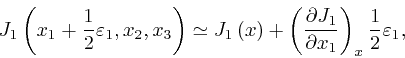
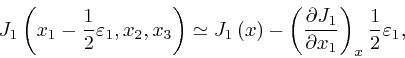
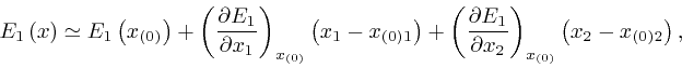
For ![]() near
near
![]() in the plane of the rectangle,
the result we obtained in the first part of the post,
here,
with
in the plane of the rectangle,
the result we obtained in the first part of the post,
here,
with
![]() taken as
taken as
![]() and
and ![]() taken as
taken as ![]() , gives:
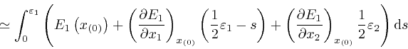
, gives:

where as the magnitudes of
![]() and
and
![]() tend to 0, the error of this approximate representation tends to
0 more rapidly than in proportion to those magnitudes.
tend to 0, the error of this approximate representation tends to
0 more rapidly than in proportion to those magnitudes.
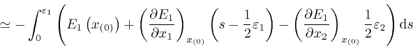
The coordinates
![]() of a point a distance
of a point a distance ![]() along the
first side of the rectangle from the first corner of this side are
along the
first side of the rectangle from the first corner of this side are
![]() . And along
this side,
. And along
this side, ![]() is equal to
is equal to ![]() plus a constant value, the length of the wire
from its first end to the first corner of this side, so
plus a constant value, the length of the wire
from its first end to the first corner of this side, so
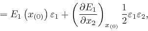
![]() . Thus since
. Thus since
![]() for this side, we have:
for this side, we have:

where the error of this approximation tends to 0 more rapidly than in
proportion to
![]() or
or
![]() as
as
![]() and
and ![]() tend to 0, and I used the result we found
in the first part of the post,
here,
that the integral of the rate of change of a quantity is equal to the
net change of that quantity, and also
tend to 0, and I used the result we found
in the first part of the post,
here,
that the integral of the rate of change of a quantity is equal to the
net change of that quantity, and also
![]() and
and
![]() ,
from the result we found in the second part of the post,
here.
,
from the result we found in the second part of the post,
here.
The coordinates
![]() of a point a distance
of a point a distance ![]() along the
third side of the rectangle from the first corner of that side are
along the
third side of the rectangle from the first corner of that side are
![]() . We again
have
. We again
have
![]() , so since
, so since
![]() for that side, we have:
for that side, we have:

to the same accuracy as before. Thus:

where the error of this approximation tends to 0 more rapidly than in
proportion to
![]() , as
, as ![]() and
and
![]() tend to 0 with their ratio fixed to a finite non-zero value.
tend to 0 with their ratio fixed to a finite non-zero value.
Similarly we find:
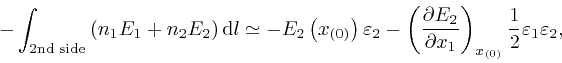
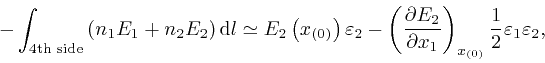
to the same accuracy. So:

to the same accuracy. Thus:
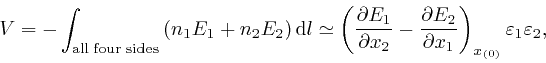
where the error of this approximation tends to 0 more rapidly than in
proportion to
![]() , as
, as ![]() and
and
![]() tend to 0 with their ratio fixed to a finite non-zero value.
tend to 0 with their ratio fixed to a finite non-zero value.
Thus from Faraday's measurements, as above:
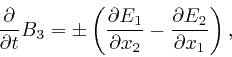
since
![]() is the area
is the area ![]() of the small rectangle. We have obtained this equation at the position
of the small rectangle. We have obtained this equation at the position
![]() of the
centre of the small rectangle, so it holds everywhere the small rectangle of
wire could have been placed.
of the
centre of the small rectangle, so it holds everywhere the small rectangle of
wire could have been placed.
To determine the sign, let's suppose that ![]() and
and ![]() are 0 at the centre
of the small rectangle, and that
are 0 at the centre
of the small rectangle, and that ![]() is positive along the 1st side of the
rectangle and negative along the 3rd side, and
is positive along the 1st side of the
rectangle and negative along the 3rd side, and ![]() is positive along the 2nd
side of the rectangle and negative along the 4th side. Then
is positive along the 2nd
side of the rectangle and negative along the 4th side. Then
![]() is negative and
is negative and
![]() is
positive, so
is
positive, so
![]() is negative, and the force
is negative, and the force
![]() on a
movable charged particle of positive
on a
movable charged particle of positive ![]() is in the direction of increasing
is in the direction of increasing ![]() along all four sides of the rectangle, so the current
along all four sides of the rectangle, so the current ![]() along the wire is
positive in the direction of increasing
along the wire is
positive in the direction of increasing ![]() .
.
From the result we found
above,
Maxwell's equation summarizing Ampère's law,
as
above,
implies that a positive current ![]() along a wire in the 3 direction
produces a magnetic induction field
along a wire in the 3 direction
produces a magnetic induction field
![]() such that
such that
![]() is negative for
is negative for ![]() greater than the
greater than the ![]() coordinate of the wire and positive otherwise, and
coordinate of the wire and positive otherwise, and
![]() is positive
for
is positive
for ![]() greater than the
greater than the ![]() coordinate of the wire and negative
otherwise.
coordinate of the wire and negative
otherwise.
The antisymmetric tensor
![]() , which I defined
above, is
unaltered by a cyclic permutation of its indexes, for example
, which I defined
above, is
unaltered by a cyclic permutation of its indexes, for example
![]() or
or
![]() , so Maxwell's equation
summarizing Ampère's law, as
above,
also implies that a positive current
, so Maxwell's equation
summarizing Ampère's law, as
above,
also implies that a positive current ![]() along a wire in the 1 direction produces a magnetic induction field
along a wire in the 1 direction produces a magnetic induction field
![]() such that
such that
![]() is positive for
is positive for ![]() greater than the
greater than the ![]() coordinate of the wire and negative otherwise, and a
positive current
coordinate of the wire and negative otherwise, and a
positive current ![]() along a wire in the 2 direction produces a magnetic
induction field
along a wire in the 2 direction produces a magnetic
induction field
![]() such that
such that
![]() is negative
for
is negative
for ![]() greater than the
greater than the ![]() coordinate of the wire and positive
otherwise.
coordinate of the wire and positive
otherwise.
Thus if the current ![]() along the wire is positive in the direction of
increasing
along the wire is positive in the direction of
increasing ![]() , the magnetic induction field
, the magnetic induction field
![]() produced by the current along
each side of the small rectangle is such that
produced by the current along
each side of the small rectangle is such that
![]() is positive inside the
small rectangle. So from the observed sign of the voltage, as I described
above,
a positive value of
is positive inside the
small rectangle. So from the observed sign of the voltage, as I described
above,
a positive value of
![]() inside the
small rectangle produces electric field strengths that result in a current
inside the
small rectangle produces electric field strengths that result in a current ![]() along the wire that is negative in the direction of increasing
along the wire that is negative in the direction of increasing ![]() , and thus
of opposite sign to those I assumed above. Thus positive
, and thus
of opposite sign to those I assumed above. Thus positive
![]() produces positive
produces positive
![]() , so the formula with the correct sign is:
, so the formula with the correct sign is:
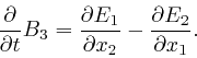
The corresponding formulae that result from considering small rectangles whose edges are in the 2 and 3 or 3 and 1 Cartesian coordinate directions are obtained from this formula by cyclic permutation of the indexes, and the three formulae can be written as:
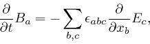
where
![]() is the totally antisymmetric tensor I defined
above.
This is Maxwell's equation summarizing Faraday's measurements involving
time-dependent magnetic fields, as
above.
is the totally antisymmetric tensor I defined
above.
This is Maxwell's equation summarizing Faraday's measurements involving
time-dependent magnetic fields, as
above.
From the discussion
above,
if the electric field strength ![]() can be derived
from a voltage field
can be derived
from a voltage field ![]() , then
, then
![]() . The electric field strength
. The electric field strength ![]() produced by the changing magnetic induction
field
produced by the changing magnetic induction
field ![]() in accordance with the above equation cannot be derived from a
voltage field
in accordance with the above equation cannot be derived from a
voltage field ![]() , for if
, for if
![]() , and
, and ![]() depends smoothly on position, then by a similar calculation to the one
above,
we have:
depends smoothly on position, then by a similar calculation to the one
above,
we have:
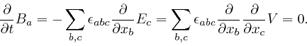
No magnetically charged particles, often referred to as magnetic monopoles, have yet been observed, and Maxwell's equation summarizing this fact, analogous to his equation summarizing Coulomb's law, as above, is:
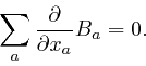
Although it's not possible to derive the electric field strength ![]() from a
voltage field
from a
voltage field ![]() alone if the magnetic induction field
alone if the magnetic induction field ![]() is time-dependent,
Maxwell's equation summarizing Faraday's measurements involving time-dependent
magnetic fields, as
above,
and his equation above summarizing the
non-observation of magnetic monopoles, can always be solved by deriving the
electric field strength
is time-dependent,
Maxwell's equation summarizing Faraday's measurements involving time-dependent
magnetic fields, as
above,
and his equation above summarizing the
non-observation of magnetic monopoles, can always be solved by deriving the
electric field strength ![]() and the magnetic induction field
and the magnetic induction field ![]() from a
voltage field
from a
voltage field ![]() and a vector field
and a vector field ![]() called the vector potential, such
that:
called the vector potential, such
that:
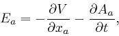
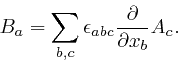
For if ![]() has this form, then the left-hand side of Maxwell's equation
summarizing Faraday's measurements involving time-dependent magnetic fields, as
above, is:
has this form, then the left-hand side of Maxwell's equation
summarizing Faraday's measurements involving time-dependent magnetic fields, as
above, is:
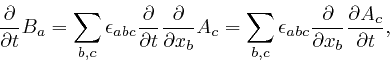
where I assumed that the vector potential ![]() depends smoothly on position and
time, and used the result we found
above.
And if
depends smoothly on position and
time, and used the result we found
above.
And if ![]() has the
above
form,
then the right-hand side of that equation is:
has the
above
form,
then the right-hand side of that equation is:
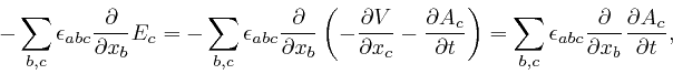
where I again used the result we found
above.
This is equal to the left-hand side
as above, so if ![]() and
and ![]() are derived from a voltage field
are derived from a voltage field ![]() and a vector
potential field
and a vector
potential field ![]() as
above,
then Maxwell's equation summarizing Faraday's
measurements involving time-dependent magnetic fields, as
above,
is solved.
as
above,
then Maxwell's equation summarizing Faraday's
measurements involving time-dependent magnetic fields, as
above,
is solved.
And if the magnetic induction field ![]() is derived from a vector potential
field
is derived from a vector potential
field ![]() as
above,
then the left-hand side of Maxwell's equation
above
summarizing the non-observation of magnetic monopoles is:
as
above,
then the left-hand side of Maxwell's equation
above
summarizing the non-observation of magnetic monopoles is:
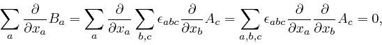
by a similar calculation to the one above. Thus Maxwell's equation summarizing the non-observation of magnetic monopoles is also solved.
If the electric field strength ![]() and the magnetic induction field
and the magnetic induction field ![]() are
derived from a voltage field
are
derived from a voltage field ![]() and a vector potential field
and a vector potential field ![]() , as
above,
then in a vacuum, where the electric displacement field
, as
above,
then in a vacuum, where the electric displacement field ![]() is related to the
electric field strength
is related to the
electric field strength ![]() by
by
![]() , and the magnetic field
strength
, and the magnetic field
strength ![]() is related to the magnetic induction field
is related to the magnetic induction field ![]() by
by
![]() , Maxwell's equation summarizing
Coulomb's law, as
above,
becomes:
, Maxwell's equation summarizing
Coulomb's law, as
above,
becomes:
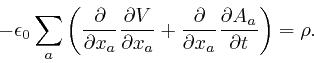
And Maxwell's corrected equation summarizing Ampère's law, as above, becomes:
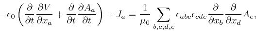
where each index
![]() from the start of the lower-case
English alphabet can take values 1, 2, 3, corresponding to the directions in
which the three Cartesian coordinates of spatial position increase.
from the start of the lower-case
English alphabet can take values 1, 2, 3, corresponding to the directions in
which the three Cartesian coordinates of spatial position increase.
To simplify the above formula, we'll consider the expression:
where ![]() is the Kronecker delta, that I defined
in the first part of the post,
here,
so its
value is 1 when
is the Kronecker delta, that I defined
in the first part of the post,
here,
so its
value is 1 when ![]() , and 0 otherwise. Thus
, and 0 otherwise. Thus
![]() , and
, and
![]() . A quantity whose value is unchanged if two
of its indexes of the same type are swapped is said to be "symmetric" in
those indexes, so from the definition of a tensor, as
above,
. A quantity whose value is unchanged if two
of its indexes of the same type are swapped is said to be "symmetric" in
those indexes, so from the definition of a tensor, as
above,
![]() is
an example of a symmetric tensor.
is
an example of a symmetric tensor.
In the
above
definition of the tensor
![]() , each term in the
right-hand side after the first term is obtained from the first term by
leaving the indexes
, each term in the
right-hand side after the first term is obtained from the first term by
leaving the indexes ![]() ,
, ![]() , and
, and ![]() in the same positions as in the first
term, and swapping the indexes
in the same positions as in the first
term, and swapping the indexes ![]() ,
, ![]() , and
, and ![]() among themselves. Among the
6 terms in the right-hand side, each of the
among themselves. Among the
6 terms in the right-hand side, each of the ![]() possible sequences of the
letters
possible sequences of the
letters ![]() occurs exactly once, where for each non-negative whole
number
occurs exactly once, where for each non-negative whole
number ![]() , I defined
, I defined ![]() in the second part of the post
here,
and we observed in the second part of the post,
here,
that the number of
different ways of putting
in the second part of the post
here,
and we observed in the second part of the post,
here,
that the number of
different ways of putting ![]() distinguishable objects in
distinguishable objects in ![]() distinguishable
places, such that exactly one object goes to each place, is
distinguishable
places, such that exactly one object goes to each place, is ![]() Thus the
number of different sequences of
Thus the
number of different sequences of ![]() different letters is
different letters is ![]() .
.
A re-ordering of a sequence of ![]() different letters is called a permutation
of the sequence. The sign of each term in the right-hand side of the
above
definition of
different letters is called a permutation
of the sequence. The sign of each term in the right-hand side of the
above
definition of
![]() is a sign associated with the permutation
that changes the sequence
is a sign associated with the permutation
that changes the sequence ![]() into the sequence in which the letters
into the sequence in which the letters ![]() occur in that term, and is defined in the following way. For any
permutation of a sequence of
occur in that term, and is defined in the following way. For any
permutation of a sequence of ![]() different letters, a cycle of the
permutation is a sequence of the letters such that the final position of each
letter of the cycle is the same as the initial position of the next letter of
the cycle, except that the final position of the last letter of the cycle is
the same as the initial position of the first letter of the cycle. For
example, for the permutation
different letters, a cycle of the
permutation is a sequence of the letters such that the final position of each
letter of the cycle is the same as the initial position of the next letter of
the cycle, except that the final position of the last letter of the cycle is
the same as the initial position of the first letter of the cycle. For
example, for the permutation
![]() , the letter
, the letter ![]() by
itself is a cycle, and
by
itself is a cycle, and ![]() is a cycle. Two cycles are considered to be
equivalent if they have the same letters, and the number of letters in a cycle
is called its length. The sign associated with a permutation, which is
called the sign of the permutation, is the sign of
is a cycle. Two cycles are considered to be
equivalent if they have the same letters, and the number of letters in a cycle
is called its length. The sign associated with a permutation, which is
called the sign of the permutation, is the sign of
![]() ,
where
,
where ![]() is the number of inequivalent cycles of even length. For example
the second term in the right-hand side of the
above
definition of
is the number of inequivalent cycles of even length. For example
the second term in the right-hand side of the
above
definition of
![]() corresponds to the permutation
corresponds to the permutation
![]() , which has just
one cycle
, which has just
one cycle ![]() whose length is 3, so its sign is
whose length is 3, so its sign is ![]() .
.
If a permutation is followed by another permutation that just swaps two
letters, then the cycles of the resulting permutation are the same as the
cycles of the original permutation, except that if the two swapped letters
were originally in the same cycle, that cycle is divided into two cycles, each
of which contains one of the swapped letters, while if the two swapped letters
were originally in two different cycles, those two cycles are combined into a
single cycle. If the two swapped letters were originally in a cycle of even
length, then when that cycle is divided into two cycles, the number of cycles
of even length either increases by 1 or decreases by 1, so
![]() is multiplied by
is multiplied by ![]() . If the two swapped letters were
originally in a cycle of odd length, then when that cycle is divided into two
cycles, one of the resulting cycles has even length and the other has odd
length, so the number of cycles of even length increases by 1, so
. If the two swapped letters were
originally in a cycle of odd length, then when that cycle is divided into two
cycles, one of the resulting cycles has even length and the other has odd
length, so the number of cycles of even length increases by 1, so
![]() is again multiplied by
is again multiplied by ![]() . And if the two swapped letters were
originally in two different cycles then the reverse of one of the preceding
cases occurs, so
. And if the two swapped letters were
originally in two different cycles then the reverse of one of the preceding
cases occurs, so
![]() is again multiplied by
is again multiplied by ![]() . Thus
swapping any two letters reverses the sign of a permutation.
. Thus
swapping any two letters reverses the sign of a permutation.
Thus if any two of the last three indexes of
![]() are swapped,
the value of
are swapped,
the value of
![]() is multiplied by
is multiplied by ![]() , so in accordance with
the definition
above,
, so in accordance with
the definition
above,
![]() is antisymmetric in its last three
indexes. Thus the value of
is antisymmetric in its last three
indexes. Thus the value of
![]() must be 0 when any two of its
last three indexes have the same value, for example
must be 0 when any two of its
last three indexes have the same value, for example
![]() must be
0, since swapping the 4th and 5th indexes of
must be
0, since swapping the 4th and 5th indexes of
![]() multiplies its
value by
multiplies its
value by ![]() . The only possible values of each index are 1, 2, or 3, so
. The only possible values of each index are 1, 2, or 3, so
![]() is 0 unless
is 0 unless
![]() is one of the
possibilities
is one of the
possibilities
![]() ,
,
![]() ,
,
![]() ,
,
![]() ,
,
![]() , or
, or
![]() , and furthermore,
, and furthermore,
From the definition of the antisymmetric tensor
![]() , as
above,
this implies that:
, as
above,
this implies that:
since this equation is true for
![]() because
because
![]() , and it is therefore also true for all
the other values of
, and it is therefore also true for all
the other values of
![]() for which
for which
![]() is
non-zero, by the preceding equation and the definition of
is
non-zero, by the preceding equation and the definition of
![]() , as
above,
and it is also true whenever two of the indexes
, as
above,
and it is also true whenever two of the indexes ![]() have the same value,
since both sides of the equation are then 0.
have the same value,
since both sides of the equation are then 0.
We can also write the definition
above of
![]() as:
as:
which is the same as the formula
above,
except that I have changed the order
of the factors in each term after the first, so that the indexes ![]() now
occur in the same order in every term, while the order of the indexes
now
occur in the same order in every term, while the order of the indexes ![]() is now different in each term. Each term now corresponds to one of the 6
permutations of the letters
is now different in each term. Each term now corresponds to one of the 6
permutations of the letters ![]() , and the sign of each term is the sign
of the corresponding permutation of the letters
, and the sign of each term is the sign
of the corresponding permutation of the letters ![]() . So in the same
way as
above,
we find that
. So in the same
way as
above,
we find that
![]() is also antisymmetric in its
first three indexes, and that:
is also antisymmetric in its
first three indexes, and that:
From this and the formula above, we find:
This is true for all ![]() cases where the indexes
cases where the indexes
![]() take values 1, 2, or 3, and from the case where
take values 1, 2, or 3, and from the case where
![]() , we find:
, we find:
Thus:
Furthermore,
![]() , since for these values of the indexes,
only the first term in the right-hand side of the
above
definition of
, since for these values of the indexes,
only the first term in the right-hand side of the
above
definition of
![]() is non-zero, and its value is 1. Thus
is non-zero, and its value is 1. Thus
![]() , so:
, so:
We now observe that:
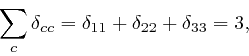
and
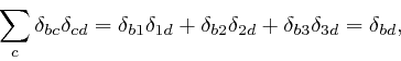
since the indexes ![]() and
and ![]() can take values 1, 2, or 3, and from the
definition of the Kronecker delta in the first part of the post,
here,
the product
can take values 1, 2, or 3, and from the
definition of the Kronecker delta in the first part of the post,
here,
the product
![]() is non-zero for exactly one value of
is non-zero for exactly one value of ![]() if
if ![]() , namely for
, namely for
![]() , in which case
, in which case
![]() , while if
, while if ![]() , where the symbol
, where the symbol ![]() means, "is not equal to," then
means, "is not equal to," then ![]() and
and ![]() are not both non-zero for any value of
are not both non-zero for any value of ![]() .
.
Thus:
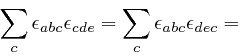

Thus Maxwell's corrected equation summarizing Ampère's law, as
above,
expressed in terms
of the voltage field ![]() and the vector potential field
and the vector potential field ![]() , as
above,
is:
, as
above,
is:
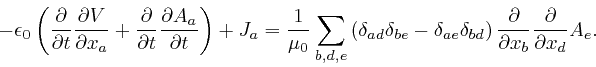
We now observe that for any vector ![]() :
:
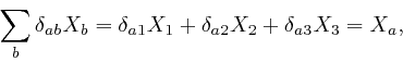
since ![]() is non-zero for exactly one value of
is non-zero for exactly one value of ![]() , namely for
, namely for ![]() , in which case it is 1.
, in which case it is 1.
Using this property of the Kronecker delta, we find:

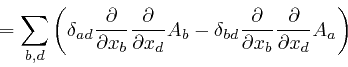
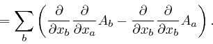
Thus Maxwell's corrected equation summarizing Ampère's law, as
above,
expressed in terms
of the voltage field ![]() and the vector potential field
and the vector potential field ![]() , as
above,
is:
, as
above,
is:
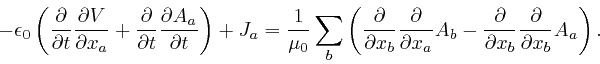
We now observe that the formulae for the electric field strength ![]() and the
magnetic induction field
and the
magnetic induction field ![]() in terms of the voltage field
in terms of the voltage field ![]() and the vector
potential field
and the vector
potential field ![]() , as
above,
are unaltered if
, as
above,
are unaltered if ![]() and
and ![]() are modified by
the following replacements:
are modified by
the following replacements:
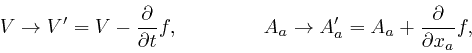
where ![]() is an arbitrary scalar field that depends smoothly on position and
time. For the modified electric field strength
is an arbitrary scalar field that depends smoothly on position and
time. For the modified electric field strength ![]() and magnetic induction
field
and magnetic induction
field ![]() are:
are:


where I used the result we found above, and a similar calculation to the one above.
The replacement of the voltage field ![]() and the vector potential field
and the vector potential field ![]() by
modified fields
by
modified fields ![]() and
and ![]() , as
above,
which leaves the electric field
strength
, as
above,
which leaves the electric field
strength ![]() and the magnetic induction field
and the magnetic induction field ![]() unaltered, and thus has no
experimentally observable consequences, is called a gauge transformation.
unaltered, and thus has no
experimentally observable consequences, is called a gauge transformation.
We can simplify Maxwell's equation summarizing Coulomb's law, and his
corrected equation summarizing Ampère's law, expressed in terms of the voltage
field ![]() and the vector potential field
and the vector potential field ![]() , as
above,
and
above,
by doing a
gauge transformation with a scalar field
, as
above,
and
above,
by doing a
gauge transformation with a scalar field ![]() that satisfies:
that satisfies:
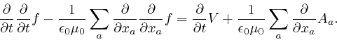
We then find that:
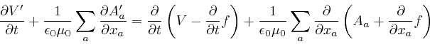
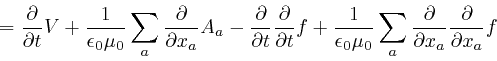
Let's now assume that we've done a gauge transformation as above, so that:
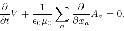
This is called a gauge condition.
Then by the result we found
above,
the term
![]() in the
left-hand side of Maxwell's equation summarizing Coulomb's law, expressed in
terms of the voltage field
in the
left-hand side of Maxwell's equation summarizing Coulomb's law, expressed in
terms of the voltage field ![]() and the vector potential field
and the vector potential field ![]() , as
above,
is equal to
, as
above,
is equal to
![]() , so that equation becomes:
, so that equation becomes:
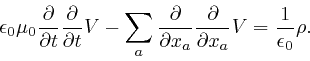
And Maxwell's corrected equation summarizing Ampère's law, expressed in terms
of the voltage field ![]() and the vector potential field
and the vector potential field ![]() , as
above,
becomes:
, as
above,
becomes:
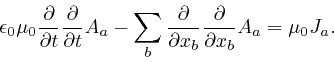
Let's now consider a region where there are no electrically charged particles
and no electric currents, so that ![]() and
and ![]() are 0. Then for any vector
are 0. Then for any vector
![]() , and any angle
, and any angle ![]() , and any vector
, and any vector ![]() perpendicular to
perpendicular to ![]() , which
from the discussion
above,
means that
, which
from the discussion
above,
means that
![]() , a solution of the
above equations that satisfies the gauge condition
above,
which we used to
simplify the equations, is given by:
, a solution of the
above equations that satisfies the gauge condition
above,
which we used to
simplify the equations, is given by:
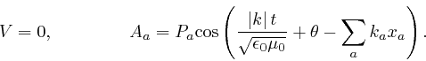
For we found in the first part of the post,
here,
that
![]() and
and
![]() . So by a calculation similar to the one
in the second part of the post,
here,
if
. So by a calculation similar to the one
in the second part of the post,
here,
if ![]() and
and ![]() are any quantities independent of
are any quantities independent of ![]() , then
, then
![]() and
and
![]() .
From these results with
.
From these results with ![]() taken as
taken as ![]() and
and ![]() , we find:
, we find:
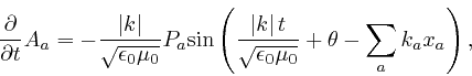
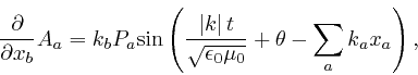
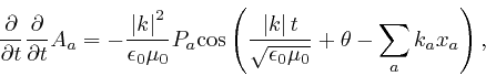
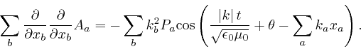
From the second of these results, we find that
![]() is proportional to
is proportional to
![]() , so
the gauge condition
above
is satisfied, and since
, so
the gauge condition
above
is satisfied, and since
![]() by Pythagoras, the third and fourth of these results show
that Maxwell's equation summarizing Ampère's law, as
above,
is satisfied. Maxwell's equation summarizing Coulomb's law, as
above,
is automatically
satisfied, since
by Pythagoras, the third and fourth of these results show
that Maxwell's equation summarizing Ampère's law, as
above,
is satisfied. Maxwell's equation summarizing Coulomb's law, as
above,
is automatically
satisfied, since ![]() for this solution.
for this solution.
From the formulae for the electric field strength ![]() and the magnetic
induction field
and the magnetic
induction field ![]() in terms of the voltage field
in terms of the voltage field ![]() and the vector potential
field
and the vector potential
field ![]() , as
above,
we find that for this solution:
, as
above,
we find that for this solution:
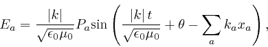
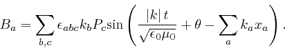
Thus since we assumed that
![]() , we find that
, we find that
![]() , which from the discussion
above
means that the vector
, which from the discussion
above
means that the vector ![]() is
perpendicular to the vector
is
perpendicular to the vector ![]() . And from calculations similar to the one
above
we find that
. And from calculations similar to the one
above
we find that
![]() , so that
, so that
![]() , so the vector
, so the vector ![]() is perpendicular to the vector
is perpendicular to the vector ![]() ,
and
,
and
![]() , so
, so
![]() , so the electric field strength
, so the electric field strength ![]() is perpendicular to the magnetic
induction field
is perpendicular to the magnetic
induction field ![]() .
.
This solution describes oscillating electric and magnetic fields moving in the
direction ![]() at a speed
at a speed
![]() . From
above,
the permittivity
. From
above,
the permittivity ![]() of a vacuum, measured from the electric charge
stored on a paralle plate capacitor, is such that:
of a vacuum, measured from the electric charge
stored on a paralle plate capacitor, is such that:
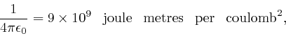
and from
above,
the definition of one amp ![]() one coulomb per second, in terms
of the force between long parallel wires carrying steady electric currents, as
above,
implies that the permeability
one coulomb per second, in terms
of the force between long parallel wires carrying steady electric currents, as
above,
implies that the permeability ![]() of a vacuum is by definition
given by:
of a vacuum is by definition
given by:
Thus:
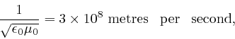
which is the measured value of the speed of light. Maxwell therefore
proposed that light is waves of oscillating electric and magnetic fields
perpendicular to the direction of motion of the wave and to each other. The
vector ![]() is called the wave vector, and the wave solutions above are called
transverse waves, because the vector potential
is called the wave vector, and the wave solutions above are called
transverse waves, because the vector potential ![]() is perpendicular to the
wave vector
is perpendicular to the
wave vector ![]() .
.
From calculations similar to those above, we find that the gauge condition above, and the field equations above, have another wave solution:
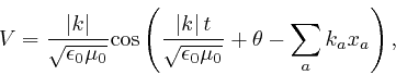
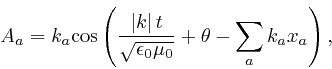
which is called a longitudinal wave, because the vector potential ![]() is
parallel to the wave vector
is
parallel to the wave vector ![]() . However from the formulae for the electric
field strength
. However from the formulae for the electric
field strength ![]() and the magnetic induction field
and the magnetic induction field ![]() in terms of the
voltage field
in terms of the
voltage field ![]() and the vector potential field
and the vector potential field ![]() , as
above,
we find that
for this solution:
, as
above,
we find that
for this solution:
Thus the above longitudinal wave solution has no experimentally observable effects. It is called a pure gauge mode.
Maxwell suggested that there could also be transverse waves of electric and magnetic fields with frequencies outside the visible spectrum, and this was partly confirmed in 1879 by experiments by David Edward Hughes, and conclusively confirmed in 1886 when Heinrich Hertz generated and detected pulses of radio-frequency electromagnetic waves in his laboratory. This led to the utilization of radio-frequency electromagnetic waves for practical communications by Guglielmo Marconi, from around 1895.
Electromagnetic waves will also be emitted by hot objects, and will be present
in a hot region that is in thermal equilibrium. It was the study of the
electromagnetic waves in hot ovens, at the end of the nineteenth century, that
provided the other part of the clue that led to the discovery of quantum
mechanics and Richard Feynman's functional integral. In the next part of this
post, Action for Fields, we'll look at how Maxwell's equations for the
for the electric
field strength ![]() and the magnetic induction field
and the magnetic induction field ![]() , expressed in terms of the
voltage field
, expressed in terms of the
voltage field ![]() and the vector potential field
and the vector potential field ![]() , as
above, can be obtained from de Maupertuis's
principle of
stationary action, for a suitable action that depends on
the electromagnetic fields
, as
above, can be obtained from de Maupertuis's
principle of
stationary action, for a suitable action that depends on
the electromagnetic fields ![]() and
and ![]() , and on the positions and motions of any
electrically charged particles present, and in the part after that,
Radiation in an Oven, we'll look at how the discoveries about heat and temperature
that we looked at in the second part
of this post, combined with the discoveries about electromagnetic radiation that
we've looked at today, lead to a seriously wrong conclusion about the properties
of electromagnetic radiation in a hot oven. In the subsequent parts of the post,
we'll look at how that problem has been resolved by the discovery of quantum
mechanics and Feynman's functional integral, which started with the identification
of a new fundamental constant of nature by
Max Planck, in 1899.
, and on the positions and motions of any
electrically charged particles present, and in the part after that,
Radiation in an Oven, we'll look at how the discoveries about heat and temperature
that we looked at in the second part
of this post, combined with the discoveries about electromagnetic radiation that
we've looked at today, lead to a seriously wrong conclusion about the properties
of electromagnetic radiation in a hot oven. In the subsequent parts of the post,
we'll look at how that problem has been resolved by the discovery of quantum
mechanics and Feynman's functional integral, which started with the identification
of a new fundamental constant of nature by
Max Planck, in 1899.
The software on this website is licensed for use under the Free Software Foundation General Public License.
Page last updated 28 November 2020. Copyright (c) Chris Austin 2012 - 2020. Privacy policy