| Home | Blog index | Previous | Next | About | Privacy policy |

By Chris Austin. 29 November 2020.
An earlier version of this post was published on another website on 17 November 2012.
This is the fourth part of a ten-part post on the foundation of our understanding of high energy physics, which is Richard Feynman's functional integral. The first three parts are Action, Multiple Molecules, and Electromagnetism, and the following parts, which will appear at intervals of about a month, are Radiation in an Oven, Matrix Multiplication, The Functional Integral, Gauge Invariance, Photons, and Interactions.
I'm hoping this blog will be fun and useful for everyone with an interest in science, so although I'll pop up a few formulae again, I'll try as usual to keep them friendly by explaining all the pieces. Please feel free to ask a question in the Comments, if you think anything in the post is unclear.
The clue that led to the discovery of quantum mechanics, whose principles are summarized in Feynman's functional integral, came from the attempted application to electromagnetic radiation of discoveries about heat and temperature. We looked at those discoveries about heat and temperature in the second part of the post, and in the third part of the post, we looked at how James Clerk Maxwell, just after the middle of the nineteenth century, was able to identify light as waves of oscillating electric and magnetic fields, and to calculate the speed of light from measurements of electrical and magnetic effects. Feynman's functional integral for a physical system depends on a property of the system called its action, and in the first part of the post, we derived Sir Isaac Newton's second law of motion from Pierre-Louis de Maupertuis's principle of stationary action.
From our study of the way heat and temperature arise from the random motions
of large numbers of microscopic objects, in the second part
of the post, the existence of a
well-defined temperature, in a region that is in thermal equilibrium, is a
consequence of the conservation of energy, which we derived in the first part
of the post, here, for a
collection of objects subject to Newton's laws of motion. The energy of a
system is related to the formula for its action, and today we'll calculate the
energy of electromagnetic fields and electrically charged particles moving in
a vacuum, by deriving Maxwell's equations summarizing
Coulomb's law and
Ampère's
law in terms of the voltage field ![]() and the vector potential field
and the vector potential field
![]() , in the forms we derived them in the third part of the post,
here and here, by de
Maupertuis's principle from an action, and we'll also derive the electrostatic
force on an electrically charged particle, as in the third part of the post,
here, and the force on a moving
charged particle from the magnetic induction field
, in the forms we derived them in the third part of the post,
here and here, by de
Maupertuis's principle from an action, and we'll also derive the electrostatic
force on an electrically charged particle, as in the third part of the post,
here, and the force on a moving
charged particle from the magnetic induction field ![]() , as in the third part of the post,
here, by de
Maupertuis's principle from that same action.
, as in the third part of the post,
here, by de
Maupertuis's principle from that same action.
From the formula for the electric field strength ![]() in terms of the voltage
field
in terms of the voltage
field ![]() and the vector potential field
and the vector potential field ![]() , in the third part of the post,
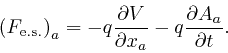
here, the formula for the
electrostatic force
, in the third part of the post,
here, the formula for the
electrostatic force
![]() on a particle of electric charge
on a particle of electric charge ![]() ,
here, becomes:
,
here, becomes:
And from the formula for the magnetic induction field ![]() in terms of the vector potential field
in terms of the vector potential field ![]() , in the third part of the post,
here, the formula
for the magnetic induction force
, in the third part of the post,
here, the formula
for the magnetic induction force
![]() on a particle of electric
charge
on a particle of electric
charge ![]() moving with velocity
moving with velocity ![]() ,
here, becomes:
,
here, becomes:
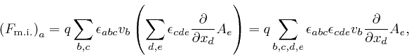
where as in the third part of the post,
here, each index
![]() from the start of the
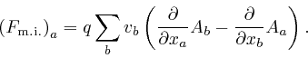
lower-case English alphabet can take values 1, 2, 3. From the formula in the third
part of the post,
here,
and a calculation similar to the one in the third part of the post,
here, this simplifies to:
from the start of the
lower-case English alphabet can take values 1, 2, 3. From the formula in the third
part of the post,
here,
and a calculation similar to the one in the third part of the post,
here, this simplifies to:
The action of a collection of electrically charged point particles moving
slowly compared to the speed of light in a vacuum, and the voltage field ![]() and the vector potential field
and the vector potential field ![]() , is:
, is:
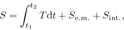
where ![]() is the kinetic energy of the particles, as in the first
part of the post,
here. The
electromagnetic action
is the kinetic energy of the particles, as in the first
part of the post,
here. The
electromagnetic action
![]() is:
is:
The integral
![]() is
over all space, and is often abbreviated to
is
over all space, and is often abbreviated to
![]() . From the formulae for the electric field strength
. From the formulae for the electric field strength ![]() and the magnetic
induction field
and the magnetic
induction field ![]() in terms of the voltage field
in terms of the voltage field ![]() and the vector potential
field
and the vector potential
field ![]() , as in the third part of the post,
here and
here, we find:
, as in the third part of the post,
here and
here, we find:
From the formula in the third part of the post, here, and a calculation similar to the one in the third part of the post, here, we find:
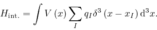
The interaction action
![]() is:
is:
where the notation is the same as we used in the first part of the post,
here,
and ![]() now represents the list of the electric charges of all the particles,
so that
now represents the list of the electric charges of all the particles,
so that ![]() is the electric charge of the
is the electric charge of the ![]() 'th particle.
'th particle.
It is convenient to let a single symbol, say ![]() , represent the entire
collection of data that includes the position data
, represent the entire
collection of data that includes the position data ![]() of all the particles at
all times, the value of the voltage field
of all the particles at
all times, the value of the voltage field ![]() at all positions and times, and
the values of the three components of the vector potential field
at all positions and times, and
the values of the three components of the vector potential field ![]() at all
positions and times. We'll let indexes
at all
positions and times. We'll let indexes
![]() distinguish the
quantities in the collection
distinguish the
quantities in the collection ![]() at each time
at each time ![]() . The possible values of
each index
. The possible values of
each index
![]() are
are ![]() , the
, the ![]() 'th position coordinate of
the
'th position coordinate of
the ![]() 'th particle;
'th particle; ![]() , the value of the voltage field at position
, the value of the voltage field at position ![]() ;
and
;
and ![]() , the value of the
, the value of the ![]() 'th component of the vector potential field
at position
'th component of the vector potential field
at position ![]() .
. ![]() or
or
![]() means the value of the
quantity
means the value of the
quantity ![]() at time
at time ![]() , so
, so
![]() ;
;
![]() ; and
; and
![]() . This sort of notation is called DeWitt's
compact index notation, after
Bryce DeWitt.
. This sort of notation is called DeWitt's
compact index notation, after
Bryce DeWitt.
A sum such as ![]() means a sum over all possible values of the index
means a sum over all possible values of the index ![]() ,
and where the possible values are continuous, as in the position index of
,
and where the possible values are continuous, as in the position index of
![]() and
and ![]() , it means an integral over the possible values. The
possible values of the index
, it means an integral over the possible values. The
possible values of the index ![]() correspond to the dynamical quantities that
can vary independently, which are called "degrees of freedom". Thus
correspond to the dynamical quantities that
can vary independently, which are called "degrees of freedom". Thus
![]() means a sum over the degrees of freedom.
means a sum over the degrees of freedom.
To extend the definition of
![]() , as in the first part of
the post,
here, to a
quantity
, as in the first part of
the post,
here, to a
quantity ![]() that depends on a collection of data such as
that depends on a collection of data such as ![]() , where the range
of possible values of an index such as
, where the range
of possible values of an index such as ![]() that distinguishes the quantities
in the collection includes continuous ranges of values, I'll first restate the
definition of
that distinguishes the quantities
in the collection includes continuous ranges of values, I'll first restate the
definition of
![]() in terms of the Kronecker
delta
in terms of the Kronecker
delta ![]() , which I defined in the first part of the
post,
here.
The range of possible values of
the indexes
, which I defined in the first part of the
post,
here.
The range of possible values of
the indexes ![]() and
and ![]() here can be any discrete range of values: the
definition of the Kronecker delta
here can be any discrete range of values: the
definition of the Kronecker delta ![]() that I used in the third part of the post,
here, where the
indexes
that I used in the third part of the post,
here, where the
indexes ![]() and
and ![]() can take values 1, 2, or 3, is a special case.
can take values 1, 2, or 3, is a special case.
In the context of the notation where ![]() represents a collection of
quantities, and the index
represents a collection of
quantities, and the index ![]() distinguishes the quantities in the collection,
the expression
distinguishes the quantities in the collection,
the expression ![]() represents the collection of quantities such that
represents the collection of quantities such that
![]() . Thus the expression
. Thus the expression
![]() represents the collection of quantities such that
represents the collection of quantities such that
![]() for
for ![]() , and
, and
![]() . Thus we can restate the definition of
. Thus we can restate the definition of
![]() , as in the first part of
the post,
here, as:
, as in the first part of
the post,
here, as:
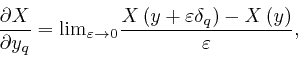
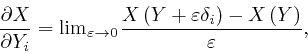
where
![]() means the limit of what
follows it, as
means the limit of what
follows it, as ![]() tends to 0. In words,
tends to 0. In words,
![]() is the rate of change of a quantity
is the rate of change of a quantity ![]() that depends on a
collection of quantities
that depends on a
collection of quantities ![]() , as the quantity
, as the quantity ![]() changes, while all the
other quantities in
changes, while all the
other quantities in ![]() have fixed values.
have fixed values.
A quantity ![]() that depends on a discrete collection of quantities
that depends on a discrete collection of quantities ![]() , some
of which can take continuous values, is sometimes said to be a function of
, some
of which can take continuous values, is sometimes said to be a function of
![]() . For example
. For example
![]() , which we studied
in the first part of the post,
here, is said to be a
function of the angle
, which we studied
in the first part of the post,
here, is said to be a
function of the angle ![]() . A quantity
. A quantity ![]() that depends on a collection
of quantities such as
that depends on a collection
of quantities such as ![]() , where the range of possible values of an index such
as
, where the range of possible values of an index such
as ![]() that distinguishes the quantities in the collection
that distinguishes the quantities in the collection ![]() includes
continuous ranges of values, is sometimes said to be a "functional" of
includes
continuous ranges of values, is sometimes said to be a "functional" of ![]() .
For example the action
.
For example the action ![]() ,
above,
is a functional of the position data
,
above,
is a functional of the position data ![]() of the particles, the voltage field
of the particles, the voltage field ![]() , and the vector potential field
, and the vector potential field ![]() .
.
To extend the definition of
![]() for a function
for a function
![]() of
of ![]() to
to
![]() for a functional
for a functional ![]() of
of ![]() ,
we'll use the analogue of the Kronecker delta
,
we'll use the analogue of the Kronecker delta ![]() for continuous
indexes, which is called the Dirac delta after
Paul Dirac. If
for continuous
indexes, which is called the Dirac delta after
Paul Dirac. If ![]() is a
quantity that can take continuous values, for example time or a position
coordinate, then the Dirac delta
is a
quantity that can take continuous values, for example time or a position
coordinate, then the Dirac delta
![]() is the limit as
is the limit as
![]() tends to 0 of a family of smooth functions
tends to 0 of a family of smooth functions
![]() of
of
![]() that have a high peak at
that have a high peak at ![]() , such that
, such that
![]() for all
for all ![]() , and
, and
![]() tends to 0 as
tends to 0 as ![]() tends to 0 for all
tends to 0 for all ![]() . For example
. For example
![]() could be
could be
 , since by a calculation
similar to the one in the second part of the post,
here, we find that
, since by a calculation
similar to the one in the second part of the post,
here, we find that
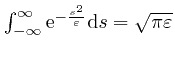 . The Dirac
delta has the property that for any function
. The Dirac
delta has the property that for any function ![]() of
of ![]() :
:
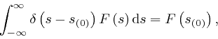
which is analogous to the property of the Kronecker delta we observed in the third part of the post, here.
We'll now extend the definition of the Kronecker delta and the Dirac delta to
the indexes
![]() that distinguish the quantities in the
collection
that distinguish the quantities in the
collection ![]() at each time
at each time ![]() in the appropriate way, using the Dirac delta
where the ranges of possible values of the indexes are continuous. Thus
we'll define
in the appropriate way, using the Dirac delta
where the ranges of possible values of the indexes are continuous. Thus
we'll define
![]() ,
,
![]() ,
,
![]() ,
,
![]() ,
,
![]() , and
, and
![]() . Here
. Here ![]() in the context
in the context ![]() or
or ![]() is understood from its context to represent a position in space,
like
is understood from its context to represent a position in space,
like ![]() in the same context. With these definitions,
in the same context. With these definitions, ![]() is 1 if
is 1 if
![]() and
and ![]() represent the same degree of freedom and 0 otherwise, and the
Kronecker delta is used in contexts where the sum
represent the same degree of freedom and 0 otherwise, and the
Kronecker delta is used in contexts where the sum ![]() means a discrete
sum, and the Dirac delta is used in contexts where it means an integral.
means a discrete
sum, and the Dirac delta is used in contexts where it means an integral.
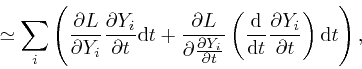
We can now define
![]() for a functional
for a functional ![]() of
of
![]() as:
as:
where in the context of the notation where ![]() represents a collection of
quantities, and the index
represents a collection of
quantities, and the index ![]() distinguishes the quantities in the collection,
the expression
distinguishes the quantities in the collection,
the expression ![]() represents the collection of quantities such that
represents the collection of quantities such that
![]() .
.
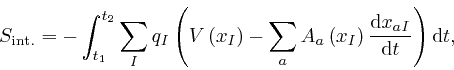
We now observe that the formula for the action ![]() ,
above, can be written as:
,
above, can be written as:
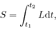
where
and
![]() and
and
![]() are the expressions that are integrated from
are the expressions that are integrated from ![]() to
to ![]() in the formulae
for
in the formulae
for
![]() ,
above, and
,
above, and
![]() above. The expression
above. The expression ![]() is called the Lagrangian, after
Joseph-Louis Lagrange,
who vigorously developed the applications of de Maupertuis's principle.
is called the Lagrangian, after
Joseph-Louis Lagrange,
who vigorously developed the applications of de Maupertuis's principle.
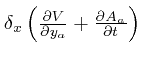
We observe, furthermore, that at each time ![]() , the expressions
, the expressions ![]() ,
,
![]() , and
, and
![]() , and
consequently also
, and
consequently also ![]() , depend on the dynamical quantities
, depend on the dynamical quantities ![]() , as
above,
only through the values of
, as
above,
only through the values of ![]() and
and
![]() at that
time
at that
time ![]() , or in other words, only through
, or in other words, only through ![]() and
and
![]() . Here I am interpreting
. Here I am interpreting
![]() as
as
![]() , since the symbol
, since the symbol
![]() is an alternative notation for
Leibniz's
is an alternative notation for
Leibniz's ![]() , as I
explained in the first part of the post,
here.
By calculations similar to those we did in the first part of the post,
here,
we find that when an action is the time integral of a
Lagrangian
, as I
explained in the first part of the post,
here.
By calculations similar to those we did in the first part of the post,
here,
we find that when an action is the time integral of a
Lagrangian ![]() , as above, such that
, as above, such that ![]() , the Lagrangian
, the Lagrangian ![]() at time
at time ![]() ,
depends on the dynamical quantities
,
depends on the dynamical quantities ![]() only through
only through ![]() and
and
![]() , the equations that result from
requiring that the action should be relatively unaltered by small changes in
the values of the dynamical quantities
, the equations that result from
requiring that the action should be relatively unaltered by small changes in
the values of the dynamical quantities ![]() and their time dependence, in
accordance with de Maupertuis's principle of stationary action, as above, are:
and their time dependence, in
accordance with de Maupertuis's principle of stationary action, as above, are:
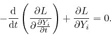
This is called Lagrange's equation. In this formula, the expressions
![]() and
and
![]() are defined by treating
are defined by treating ![]() and
and
![]() as completely independent
quantities. The change to the action that results from the replacement of
as completely independent
quantities. The change to the action that results from the replacement of
![]() by
by
![]() , where
, where
![]() is small for all
is small for all ![]() and
all
and
all ![]() , is the time integral of the sum
, is the time integral of the sum ![]() of
of ![]() times the
left-hand side of the above equation, plus terms that tend to 0 more rapidly
than in proportion to
times the
left-hand side of the above equation, plus terms that tend to 0 more rapidly
than in proportion to ![]() , as
, as ![]() tends to 0.
tends to 0.
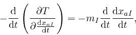
We'll now use Lagrange's equation, as above, to find the equations that result
from the application of de Maupertuis's principle to the action ![]() ,
above. For
,
above. For
![]() , we find from the formula for the kinetic energy
, we find from the formula for the kinetic energy
![]() of the particles, as in the first part of the post,
here, that:
of the particles, as in the first part of the post,
here, that:
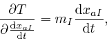
where I used Leibniz's rule for the rate of change of a product, which we obtained in the first part of the post, here. Thus:
which is in agreement with the result we found in the first part of the post,
here. ![]() does not depend on
does not depend on ![]() other than through
other than through
![]() , and from the formula for
, and from the formula for
![]() ,
above,
,
above,
![]() does not depend on
does not depend on ![]() or
or
![]() . From the formula for
. From the formula for
![]() ,
above, we find:
,
above, we find:
For the first of the above two formulae, I rewrote the dummy index ![]() that is
summed over by
that is
summed over by ![]() in the formula for
in the formula for
![]() as
as ![]() , to avoid confusing it
with the index
, to avoid confusing it
with the index ![]() on the quantity
on the quantity ![]() we are evaluating the rate of
change of
we are evaluating the rate of
change of
![]() with respect to.
with respect to.
To calculate
 , we observe that by the result we found in the first
part of the post,
here, with
, we observe that by the result we found in the first
part of the post,
here, with ![]() taken as
taken as
![]() , and the
, and the ![]() taken as
taken as ![]() ,
, ![]() ,
, ![]() , and
, and ![]() , we
have:
, we
have:
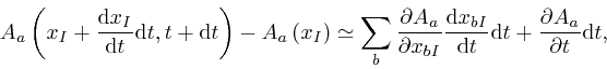
where the error of this approximate representation tends to 0 more rapidly
than in proportion to ![]() , as
, as ![]() tends to 0. For a
formula such as this one, where we have not yet divided the change during time
tends to 0. For a
formula such as this one, where we have not yet divided the change during time
![]() by
by ![]() , we relax the rule that Leibniz's
, we relax the rule that Leibniz's
![]() means that the formula is to be taken in the limit where
means that the formula is to be taken in the limit where
![]() tends to 0, because the formula would otherwise give
tends to 0, because the formula would otherwise give ![]() . On dividing the above formula by
. On dividing the above formula by ![]() , and then taking the limit
where
, and then taking the limit
where ![]() tends to 0, we find:
tends to 0, we find:
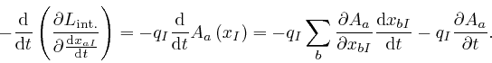
Thus from Lagrange's equation, above, we have:

Rearranging this formula as:
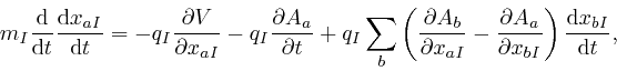
we recognize it as:
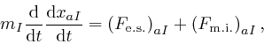
where
![]() is the electrostatic force, as
above, on the
is the electrostatic force, as
above, on the ![]() 'th particle, and
'th particle, and
![]() is the
magnetic induction force, as
above, on the
is the
magnetic induction force, as
above, on the ![]() 'th particle.
'th particle.
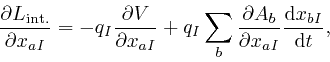
For ![]() ,
, ![]() gives no contribution. From the formula for
gives no contribution. From the formula for
![]() ,
above, we find:
,
above, we find:

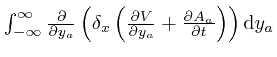
In the second line here, I rewrote the dummy position index ![]() that is
integrated over by
that is
integrated over by
![]() in the formula for
in the formula for
![]() as
as ![]() , to avoid confusing it with the index
, to avoid confusing it with the index ![]() on the
quantity
on the
quantity ![]() we are evaluating the rate of change of
we are evaluating the rate of change of
![]() with respect to.
with respect to. ![]() means
means
![]() ,
in accordance with the definitions
above and
above.
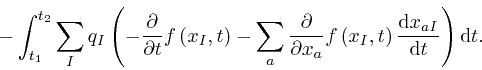
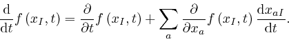
The fourth line is obtained from the third
line in a similar manner to the calculation in the first part of the post,
here: we use
Leibniz's rule for
the rate of change of a product to calculate the rate of change of the product
,
in accordance with the definitions
above and
above.
The fourth line is obtained from the third
line in a similar manner to the calculation in the first part of the post,
here: we use
Leibniz's rule for
the rate of change of a product to calculate the rate of change of the product
 with respect to
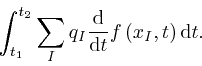
 ![]() , then use the result that the
integral
, then use the result that the
integral
 is the difference between the value of
as
is the difference between the value of
as ![]() tends to
tends to ![]() and its value as
and its value as ![]() tends to
tends to ![]() , which is 0, since
, which is 0, since
![]() is 0
in both these limits. And the fifth line is obtained from the fourth line by
using the result
above for the Dirac delta, with
is 0
in both these limits. And the fifth line is obtained from the fourth line by
using the result
above for the Dirac delta, with ![]() taken as
taken as ![]() and
and
![]() taken as
taken as ![]() , for
, for ![]() .
.
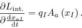
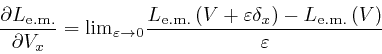
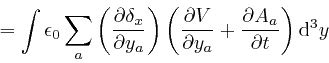
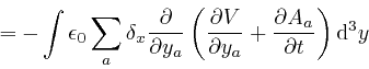
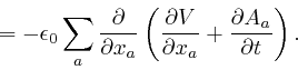
From the formula for
![]() ,
above, we also find:
,
above, we also find:

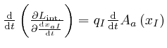
From the formula for
![]() ,
above,
we find:
,
above,
we find:
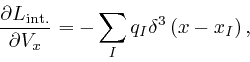
where
![]() , and:
, and:

Thus from Lagrange's equation, above, we find:
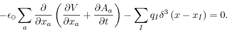
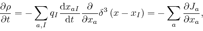
This is in agreement with Maxwell's equation summarizing Coulomb's law, as
in the third part of this post,
here,
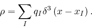
since for a collection of point particles at positions ![]() with
electric charges
with
electric charges ![]() , the electric charge density
, the electric charge density ![]() is:
is:
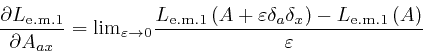
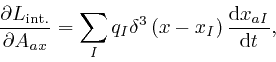
For
![]() ,
, ![]() again gives no contribution. From the
formula for
again gives no contribution. From the
formula for
![]() ,
above, two terms in
,
above, two terms in
![]() give
contributions to
give
contributions to
![]() , namely
the term involving
, namely
the term involving
![]() , which I shall call
, which I shall call
![]() , and the term
involving
, and the term
involving
![]() , which I shall call
, which I shall call
![]() . We find:
. We find:
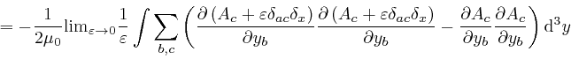
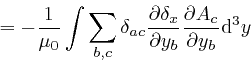
where the successive steps are as in the corresponding calculation for ![]() , as
above,
and in the fourth line I also used the result we observed in the third part of the
post,
here,
for the Kronecker delta. And similarly:
, as
above,
and in the fourth line I also used the result we observed in the third part of the
post,
here,
for the Kronecker delta. And similarly:
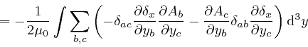
where the successive steps are the same again, and in going from the fourth
line to the fifth line, I rewrote the dummy index ![]() in the second term in
the fourth line as
in the second term in
the fourth line as ![]() .
.
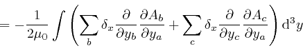
From the formula for
![]() ,
above, we also find:
,
above, we also find:
Thus:
From the formula for
![]() ,
above,
we find:
,
above,
we find:

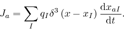
Thus from Lagrange's equation, above, we find:

This is in agreement with Maxwell's equation summarizing Ampère's law, as
in the third part of this post,
here,
since for a collection of point particles at positions ![]() with
electric charges
with
electric charges ![]() , the electric current density
, the electric current density ![]() is:
is:
As a check of this formula for ![]() , we observe that for the electric charge
density
, we observe that for the electric charge
density ![]() of a collection of point particles at positions
of a collection of point particles at positions ![]() with
electric charges
with
electric charges ![]() , as
above,
the result we found in the first part of this post,
here, with
, as
above,
the result we found in the first part of this post,
here, with ![]() taken as
taken as
![]() and the
and the ![]() taken as
taken as ![]() , gives:
, gives:
where the error of this approximate representation tends to 0 more rapidly
than in proportion to ![]() , as
, as ![]() tends to 0. Thus:
tends to 0. Thus:
where the electric current density ![]() is as
above.
Thus the electric charge density
is as
above.
Thus the electric charge density ![]() of a collection of point particles at positions
of a collection of point particles at positions ![]() with electric charges
with electric charges ![]() , as
above,
and the electric current density
, as
above,
and the electric current density ![]() of those particles, as
above,
satisfy the equation expressing the conservation
of electric charge, as in the third part of this post,
here.
of those particles, as
above,
satisfy the equation expressing the conservation
of electric charge, as in the third part of this post,
here.
Thus for a collection of electrically charged point particles moving slowly
compared to the speed of light in a vacuum, the electrostatic force
![]() on those particles, as
above,
the magnetic induction force
on those particles, as
above,
the magnetic induction force
![]() on those particles, as
above,
Maxwell's equation
summarizing Coulomb's law, as in the third part of this post,
here,
and Maxwell's equation summarizing
Ampère's law, as in the third part of this post,
here,
all follow from the application of de Maupertuis's
principle of stationary action, as in the first part of the post,
here, to the action
on those particles, as
above,
Maxwell's equation
summarizing Coulomb's law, as in the third part of this post,
here,
and Maxwell's equation summarizing
Ampère's law, as in the third part of this post,
here,
all follow from the application of de Maupertuis's
principle of stationary action, as in the first part of the post,
here, to the action ![]() ,
above. And
Maxwell's equation summarizing
Faraday's
measurements involving time-dependent
magnetic fields, as in the third part of the post,
here,
and Maxwell's equation above summarizing the
non-observation of magnetic monopoles, as in the third part of the post,
here, are automatically satisfied,
due to the formulae expressing the electric field strength
,
above. And
Maxwell's equation summarizing
Faraday's
measurements involving time-dependent
magnetic fields, as in the third part of the post,
here,
and Maxwell's equation above summarizing the
non-observation of magnetic monopoles, as in the third part of the post,
here, are automatically satisfied,
due to the formulae expressing the electric field strength ![]() and the
magnetic induction field
and the
magnetic induction field ![]() in terms of the voltage field
in terms of the voltage field ![]() and the vector
potential field
and the vector
potential field ![]() , as in the third part of the post,
here.
, as in the third part of the post,
here.
We observe that the action ![]() ,
above,
is unaltered when the voltage field
,
above,
is unaltered when the voltage field ![]() and the vector potential field
and the vector potential field ![]() are changed by a gauge transformation, as
in the third part of this post,
here,
if the scalar field
are changed by a gauge transformation, as
in the third part of this post,
here,
if the scalar field ![]() that defines the gauge transformation is 0 at
the times
that defines the gauge transformation is 0 at
the times ![]() and
and ![]() between which the action is calculated. For the
first form of the formula for
between which the action is calculated. For the
first form of the formula for
![]() , as
above, shows that
, as
above, shows that
![]() only depends on
only depends on ![]() and
and ![]() through the electric field
strength
through the electric field
strength ![]() and the magnetic induction field
and the magnetic induction field ![]() , which are unchanged by the
gauge transformation, as we found in the third part of the post,
here. And the change to
, which are unchanged by the
gauge transformation, as we found in the third part of the post,
here. And the change to
![]() ,
above,
that results from the gauge transformation, is:
,
above,
that results from the gauge transformation, is:
The result we found in the first part of the post,
here, with ![]() taken as
taken as ![]() , and the
, and the ![]() taken as the
taken as the
![]() and
and ![]() , gives:
, gives:

where the error of this approximate representation tends to 0 more rapidly
than in proportion to ![]() , as
, as ![]() tends to 0. So:
tends to 0. So:
Thus the formula
above
for the change to
![]() , that results from the gauge
transformation, is:
, that results from the gauge
transformation, is:
So from the result we found in the first part of the post,
here,
that the integral of the rate of change of
a quantity is equal to the net change of that quantity, the change to
![]() , that results from the gauge
transformation, is 0 if
, that results from the gauge
transformation, is 0 if ![]() is 0 at
is 0 at ![]() and
and ![]() . Thus since
. Thus since ![]() , the
kinetic energy of the particles, does not depend on
, the
kinetic energy of the particles, does not depend on ![]() or
or ![]() , the action
, the action ![]() is unaltered by the gauge transformation, if
is unaltered by the gauge transformation, if ![]() is 0 at
is 0 at ![]() and
and ![]() . This property of
. This property of ![]() is called gauge invariance.
is called gauge invariance.
For any system whose action, ![]() , can be expressed in terms of a Lagrangian,
, can be expressed in terms of a Lagrangian,
![]() , as
above,
such that
, as
above,
such that ![]() , the Lagrangian at time
, the Lagrangian at time ![]() , depends on the
dynamical quantities
, depends on the
dynamical quantities ![]() only through
only through ![]() and
and
![]() , the values of
, the values of ![]() and
and
![]() at the time
at the time ![]() , so that de Maupertuis's principle of
stationary action leads to Lagrange's equation, as
above,
the following expression:
, so that de Maupertuis's principle of
stationary action leads to Lagrange's equation, as
above,
the following expression:
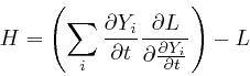
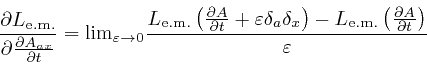
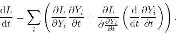
is automatically independent of time. For by Leibniz's rule for the rate of change of a product, which we obtained in the first part of the post, here:
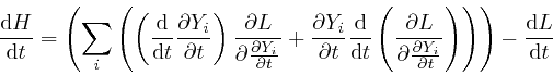
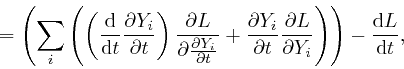
where the second line follows from Lagrange's equation,
above.
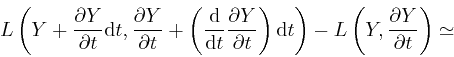
And from the result we found in the first part of the post,
here, with ![]() taken as
taken as ![]() , and the quantities
, and the quantities ![]() taken
as the quantities
taken
as the quantities ![]() and
and
![]() , we have:
, we have:
where the error of this approximation tends to 0 more rapidly than in
proportion to ![]() , as
, as ![]() tends to 0. Thus:
tends to 0. Thus:
So from the formula above:

For a system that includes a collection of point particles, so that ![]() includes a term that is the kinetic energy
includes a term that is the kinetic energy ![]() of those particles, as
above,
the formula for
of those particles, as
above,
the formula for
![]() , as
above,
shows that
, as
above,
shows that
![]() , so that
, so that ![]() also includes a term
also includes a term ![]() . Thus
. Thus ![]() must be the total energy of the system, and the result that
must be the total energy of the system, and the result that
![]() , so that the value of
, so that the value of ![]() is
independent of time, expresses the conservation of energy.
is
independent of time, expresses the conservation of energy. ![]() is called the
Hamiltonian of the system, after
Sir William Rowan Hamilton.
is called the
Hamiltonian of the system, after
Sir William Rowan Hamilton.
From the formulae for the action, ![]() , as
above,
, as
above,
![]() , as
above,
, as
above,
![]() , as
above,
, as
above,
![]() , as
above, and
, as
above, and
![]() , as
above,
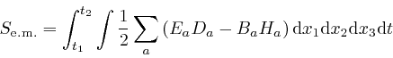
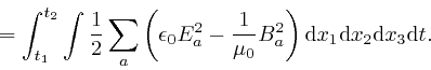
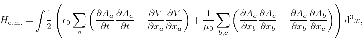
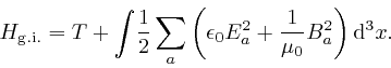
we find that the Hamiltonian for a collection of electrically charged point
particles moving slowly compared to the speed of light in a vacuum, and the
voltage field
, as
above,
we find that the Hamiltonian for a collection of electrically charged point
particles moving slowly compared to the speed of light in a vacuum, and the
voltage field ![]() and the vector potential field
and the vector potential field ![]() , is:
, is:
where ![]() is the kinetic energy of the particles, as
in the first part of the post,
here,
is the kinetic energy of the particles, as
in the first part of the post,
here,
and
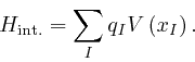
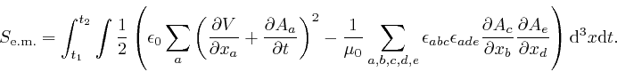
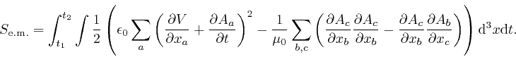
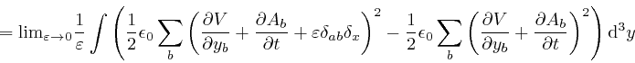
The above formula for ![]() is not manifestly left unchanged by the gauge
transformations that modify the voltage field
is not manifestly left unchanged by the gauge
transformations that modify the voltage field ![]() and the vector potential
field
and the vector potential
field ![]() , as in the third part of the post,
here,
but leave the electric field strength
, as in the third part of the post,
here,
but leave the electric field strength ![]() and the
magnetic induction field
and the
magnetic induction field ![]() unaltered, and thus have no experimentally
observable consequences. However by the property of the Dirac delta we
observed
above,
we can write
unaltered, and thus have no experimentally
observable consequences. However by the property of the Dirac delta we
observed
above,
we can write
![]() ,
above, as:
,
above, as:
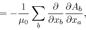
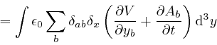
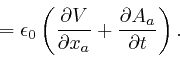
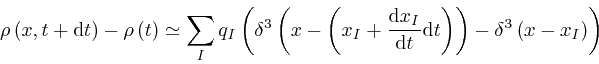
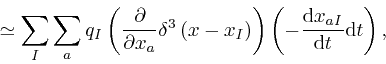
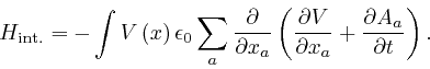
So when Maxwell's equation summarizing Coulomb's law, as above, is satisfied, we have:
When the number of electrically charged point particles is finite, ![]() and
and ![]() tend to 0 when any of the position coordinates
tend to 0 when any of the position coordinates ![]() tend to
tend to ![]() , so
by a calculation similar to the way we obtained the fourth line from the third
line in the calculation
above,
we find:
, so
by a calculation similar to the way we obtained the fourth line from the third
line in the calculation
above,
we find:
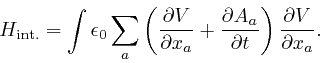
Thus:
where the second line here follows from reversing the steps that led from the
first version of the formula for
![]() , as
above,
to the final version, as
above.
, as
above,
to the final version, as
above.
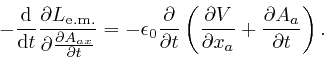
Thus when the Lagrange equation that follows from the application of de
Maupertuis's principle to the action ![]() ,
above,
is satisfied, the Hamiltonian
,
above,
is satisfied, the Hamiltonian
![]() ,
above,
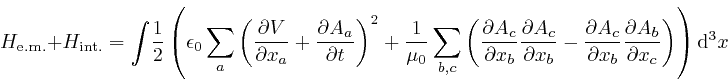
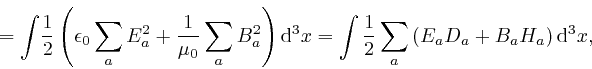
is equal to the gauge invariant Hamiltonian:
,
above,
is equal to the gauge invariant Hamiltonian:
Thus since
![]() when the Lagrange equation
is satisfied, we also have
when the Lagrange equation
is satisfied, we also have
 when the Lagrange equation is satisfied.
![]() is the
manifestly gauge invariant formula for the total energy of a collection of
electrically charged point particles moving slowly compared to the speed of
light in a vacuum, and the electric field strength
is the
manifestly gauge invariant formula for the total energy of a collection of
electrically charged point particles moving slowly compared to the speed of
light in a vacuum, and the electric field strength ![]() and the magnetic
induction field
and the magnetic
induction field ![]() .
.
In the next part of this
post, Radiation in an Oven, we'll use the above formula for
![]() to look at how the discoveries about heat and temperature
that we looked at in the second part
of this post, combined with the discoveries about electromagnetic radiation that
we looked at in the
third part
of the post, lead to a seriously wrong conclusion about the properties
of electromagnetic radiation in a hot oven. In the subsequent parts of the post,
we'll look at how that problem has been resolved by the discovery of quantum
mechanics and Feynman's functional integral, which started with the identification
of a new fundamental constant of nature by
Max Planck, in 1899.
to look at how the discoveries about heat and temperature
that we looked at in the second part
of this post, combined with the discoveries about electromagnetic radiation that
we looked at in the
third part
of the post, lead to a seriously wrong conclusion about the properties
of electromagnetic radiation in a hot oven. In the subsequent parts of the post,
we'll look at how that problem has been resolved by the discovery of quantum
mechanics and Feynman's functional integral, which started with the identification
of a new fundamental constant of nature by
Max Planck, in 1899.
The software on this website is licensed for use under the Free Software Foundation General Public License.
Page last updated 29 November 2020. Copyright (c) Chris Austin 2012 - 2020. Privacy policy