| Home | Blog index | Previous | Next | About | Privacy policy |
By Chris Austin. 26 November 2020.
An earlier version of this post was published on another website on 26 July 2012.
Hello, and welcome to this blog. I am Chris Austin, I work independently on high energy physics theory, in Maryport on the north-west coast of England, UK.
In this series of posts, I would like to tell you something about the foundation of our understanding of the way the physical world works, which I'll call Dirac-Feynman-Berezin sums.
I'll show you some formulae and things like that along the way, but I'll try to explain what all the parts mean as we go along, so you don't need to know about that sort of thing in advance.
First I have to tell you about action.
About 60 years after Sir Isaac Newton published his laws of motion in 1687, Pierre-Louis Moreau de Maupertuis discovered that Newton's laws follow from the requirement that a quantity he called "action", that depends on the positions and motions of a collection of objects over a period of time, should be relatively unaltered by small changes in the positions and motions of those objects.
For an example, let's consider a collection of objects, such that each object
behaves approximately as though its mass is concentrated at a single point,
the objects are moving slowly compared to the speed of light, and the forces
between the objects arise from a contribution to their total energy, called
their potential energy ![]() , that depends on their positions but not on their
motions. This is a useful first approximation for many things in the
everyday world, for the Sun and the planets in the Solar System, for the
motions of most of the stars in our galaxy, and for the atoms in a solid,
liquid, gas, or living thing.
, that depends on their positions but not on their
motions. This is a useful first approximation for many things in the
everyday world, for the Sun and the planets in the Solar System, for the
motions of most of the stars in our galaxy, and for the atoms in a solid,
liquid, gas, or living thing.
If ![]() denotes the sum of the kinetic energies of the objects, or in other
words, the energy due to their motion, where the kinetic energy of a pointlike
object of mass
denotes the sum of the kinetic energies of the objects, or in other
words, the energy due to their motion, where the kinetic energy of a pointlike
object of mass ![]() moving at a speed
moving at a speed ![]() is
is
![]() if
if ![]() is small
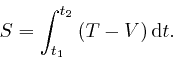
compared to the speed of light, then the formula for the action of the objects
over a period of time that begins at
is small
compared to the speed of light, then the formula for the action of the objects
over a period of time that begins at ![]() and ends at
and ends at ![]() is:
is:
 means that
 We can specify the position of an object at a particular moment in time by 3 numbers, called coordinates. For example, we can specify the position of an aeroplane by its latitude and longitude, in degrees, and its altitude, in meters. We can write these 3 numbers as a list, for example (latitude, longitude, altitude).
If the number of objects in our example is ![]() , then their positions, at a
particular moment in time, can be specified by a table of numbers with 3
columns and
, then their positions, at a
particular moment in time, can be specified by a table of numbers with 3
columns and ![]() rows. Each row gives the coordinates of a different one of the
objects. The motions of the
rows. Each row gives the coordinates of a different one of the
objects. The motions of the ![]() objects over a period of time can be
represented as accurately as desired by a series of such tables, one for each
of a closely spaced sequence of moments in time.
objects over a period of time can be
represented as accurately as desired by a series of such tables, one for each
of a closely spaced sequence of moments in time.
It is convenient to let a single symbol, say ![]() , represent this entire
collection of data. Then if the letter
, represent this entire
collection of data. Then if the letter ![]() , for example, represents one of
the numbers 1, 2, 3, and the letter
, for example, represents one of
the numbers 1, 2, 3, and the letter ![]() , for example, represents one of the
numbers
, for example, represents one of the
numbers
![]() , the value of position coordinate number
, the value of position coordinate number ![]() , of
object number
, of
object number ![]() , at time
, at time ![]() , can be represented as
, can be represented as ![]() , where the
subscripts
, where the
subscripts ![]() ,
, ![]() , and
, and ![]() are called indexes. Alternative notations for
the same thing, which can be used as convenient, are
are called indexes. Alternative notations for
the same thing, which can be used as convenient, are
![]() , and
, and
![]() , for example.
, for example.
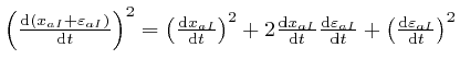
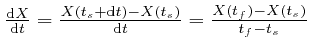
The speed ![]() of an object is proportional to the rate at which its
coordinates change with time. If a collection of data that gives the value
of a quantity at each moment in time is represented by a symbol or expression
of an object is proportional to the rate at which its
coordinates change with time. If a collection of data that gives the value
of a quantity at each moment in time is represented by a symbol or expression
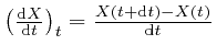
![]() , then the collection of data that gives the rate of change of that
quantity with time, at each moment in time, is often represented as
, then the collection of data that gives the rate of change of that
quantity with time, at each moment in time, is often represented as
![]() , or alternatively
, or alternatively
![]() . The Leibniz
. The Leibniz ![]() in the
numerator of
in the
numerator of
![]() means, "the change in the
following expression, when the time changes by the tiny amount
means, "the change in the
following expression, when the time changes by the tiny amount ![]() ," and indicates that the formula is to be taken in the limit where the
size of the time interval
," and indicates that the formula is to be taken in the limit where the
size of the time interval ![]() tends to 0. The value of
tends to 0. The value of
![]() at time
at time ![]() is
is
 , which is well-defined if
 ![]() changes
smoothly with
changes
smoothly with ![]() . The coordinates
. The coordinates ![]() of the objects in our example
will change smoothly with
of the objects in our example
will change smoothly with ![]() for a sensible choice of position coordinates,
since we assumed that
for a sensible choice of position coordinates,
since we assumed that ![]() is small compared to the speed of light, and thus
finite.
is small compared to the speed of light, and thus
finite.
To calculate the speed ![]() of object number
of object number ![]() , we need to know to the
distance travelled for a small change in its coordinates
, we need to know to the
distance travelled for a small change in its coordinates ![]() . For
example the distance travelled by an aeroplane, for a
. For
example the distance travelled by an aeroplane, for a ![]() change in
its longitude at fixed latitude and altitude, is smaller, the closer the
aeroplane is to the north or south pole.
change in
its longitude at fixed latitude and altitude, is smaller, the closer the
aeroplane is to the north or south pole.
For the flat 2-dimensional world of Euclidean geometry, we can choose as
coordinates the distances from 2 fixed straight lines, at right-angles to one
another. These coordinates were introduced by
René Descartes,
and are called
Cartesian coordinates. The distance ![]() between two points whose
between two points whose ![]() coordinates differ by
coordinates differ by ![]() and whose
and whose ![]() coordinates differ by
coordinates differ by ![]() is then
given by Pythagoras as
is then
given by Pythagoras as
![]() , since directly from the
diagram,
, since directly from the
diagram,
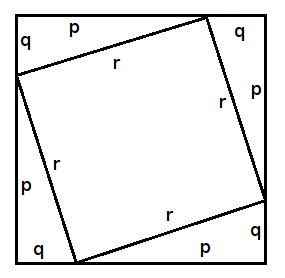
![]() .
.
For the flat 3-dimensional generalization of Euclidean geometry, called
3-dimensional Euclidean space, we can choose as coordinates the distances from
3 fixed flat planes, each at right-angles to the other two. These are also
called Cartesian coordinates. The distance ![]() between two points whose
between two points whose
![]() coordinates differ by
coordinates differ by ![]() , for
, for ![]() and
and ![]() , is then
, is then
![]() , which follows from applying Pythagoras first to
the
, which follows from applying Pythagoras first to
the ![]() and
and ![]() coordinates, and then to
coordinates, and then to
![]() and
and ![]() .
.
The assumptions of our example imply that any gravitational fields present are
sufficiently weak that if we use Cartesian coordinates, then distances are
given by Pythagoras to a good approximation, for otherwise the objects would
not continue to move slowly compared to the speed of light. Then in
Cartesian coordinates, the speed ![]() of object number
of object number ![]() is
is
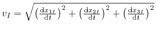 , and the sum of the kinetic energies of the
objects is given by:
, and the sum of the kinetic energies of the
objects is given by:
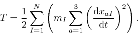
The symbol ![]() is the upper-case Greek letter Sigma, and indicates a sum of
what follows it. The idea is that each contribution to the sum is obtained
from the expression that follows the
is the upper-case Greek letter Sigma, and indicates a sum of
what follows it. The idea is that each contribution to the sum is obtained
from the expression that follows the ![]() , by substituting a specific value
for one of the indexes in the expression, and the notations below and above
the
, by substituting a specific value
for one of the indexes in the expression, and the notations below and above
the ![]() show which index is to be substituted, and the range of values of
that index, for which terms are to be included in the sum. Thus the meaning
of
show which index is to be substituted, and the range of values of
that index, for which terms are to be included in the sum. Thus the meaning
of ![]() is quite similar to the meaning of
is quite similar to the meaning of ![]() as above. The difference is that
as above. The difference is that
![]() is used for a sum over a discrete index such as
is used for a sum over a discrete index such as ![]() or
or ![]() , while
, while
![]() , together with a tiny factor such as
, together with a tiny factor such as ![]() , is used for a sum
over a continuous index such as
, is used for a sum
over a continuous index such as ![]() .
.
Let's now consider a small change to the positions and motions of the ![]() objects during the period of time from
objects during the period of time from ![]() to
to ![]() . I'll represent the
change, or "perturbation", of the positions and motions by the Greek letter
. I'll represent the
change, or "perturbation", of the positions and motions by the Greek letter
![]() , pronounced epsilon, which is often used to represent a small
quantity, so the modified positions and motions are represented by
, pronounced epsilon, which is often used to represent a small
quantity, so the modified positions and motions are represented by
![]() . Here
. Here ![]() , like
, like ![]() , represents an entire collection
of data, for example it could introduce different types of wobbles to the
motions of each of the objects. I shall assume that
, represents an entire collection
of data, for example it could introduce different types of wobbles to the
motions of each of the objects. I shall assume that ![]() is 0 at
is 0 at
![]() and
and ![]() , or in other words, that
, or in other words, that
![]() for all values
for all values ![]() of
of ![]() and all values
and all values
![]() of
of ![]() , while for times
, while for times ![]() between
between ![]() and
and
![]() , I shall assume only that all the
, I shall assume only that all the
![]() are small, and
change smoothly with time.
are small, and
change smoothly with time.
Near the start of the post, above,
I said that de Maupertuis's requirement, which
implies Newton's laws, is that the action should be relatively unaltered by
small changes to the positions and motions of the objects. What I meant by
that is that as ![]() tends to 0, or in other words, as
tends to 0, or in other words, as
![]() approaches 0 for all relevant values of
approaches 0 for all relevant values of ![]() ,
, ![]() , and
, and
![]() , the change to the action should tend to 0 more rapidly than in proportion
to
, the change to the action should tend to 0 more rapidly than in proportion
to ![]() .
.
The change to the contribution
 to the
action, that results from the replacement of
to the
action, that results from the replacement of ![]() by
by
![]() , is:
, is:
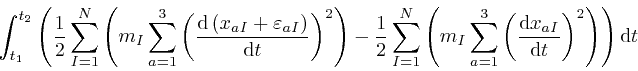
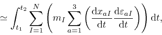
 , and the contribution from the first expression,
usually called a term, in the right-hand side of this, cancels against the
last expression in the left-hand side of the above equation for each value of
the indexes
, and the contribution from the first expression,
usually called a term, in the right-hand side of this, cancels against the
last expression in the left-hand side of the above equation for each value of
the indexes
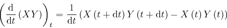
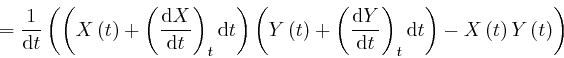
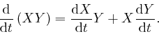
Let's now consider the rate of change with time of a product ![]() , where
, where
![]() and
and ![]() represent collections of data that give the values, at each moment
in time, of quantities that change smoothly with time. The expression
represent collections of data that give the values, at each moment
in time, of quantities that change smoothly with time. The expression ![]() represents the collection of data that gives the value of the product
represents the collection of data that gives the value of the product ![]() at each moment in time, so from above, the collection of data that gives
the rate of change with time of the product
at each moment in time, so from above, the collection of data that gives
the rate of change with time of the product ![]() , at each moment in time,
can be represented as
, at each moment in time,
can be represented as
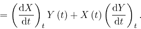
![]() . And:
. And:
 , we have
 is 0 in the limit where
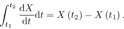
The above formula is true at every value of the time ![]() , so it can be
summarized as:
, so it can be
summarized as:
Applying this to the product
![]() , we have:
, we have:
 that results from the replacement of
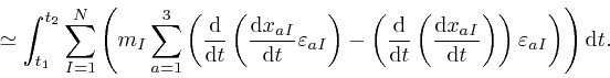
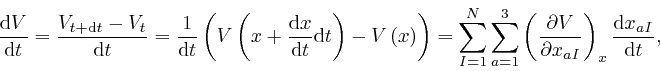
Let's now consider the expression
 , where
 ![]() is any time-dependent quantity whose
value
is any time-dependent quantity whose
value ![]() changes smoothly with time. From the description I gave near the
start of the post above,
this expression is given by dividing the period from
changes smoothly with time. From the description I gave near the
start of the post above,
this expression is given by dividing the period from ![]() to
to ![]() up into a great number of tiny time intervals, each so small that
up into a great number of tiny time intervals, each so small that
![]() only changes by a tiny amount during any
one time interval, and adding together a contribution from each of these tiny
time intervals. The contribution from a tiny time interval of length
only changes by a tiny amount during any
one time interval, and adding together a contribution from each of these tiny
time intervals. The contribution from a tiny time interval of length
![]() is
is
![]() , where
, where
![]() is evaluated at an arbitrary moment during
that interval, and the expression is the limit of the sum of all the
contributions, as the period is divided up so finely that the length of the
longest tiny interval tends to 0.
is evaluated at an arbitrary moment during
that interval, and the expression is the limit of the sum of all the
contributions, as the period is divided up so finely that the length of the
longest tiny interval tends to 0.
For a tiny time interval that starts at time ![]() and finishes at time
and finishes at time ![]() ,
where
,
where
![]() , we have
, we have
 in the
limit where
in the
limit where ![]() tends to 0, so the contribution of that interval is
tends to 0, so the contribution of that interval is
![]() . When
we add together the contributions of all the tiny
intervals, the
. When
we add together the contributions of all the tiny
intervals, the
![]() term in the contribution of each
interval except the last one cancels the
term in the contribution of each
interval except the last one cancels the
![]() term in the
contribution of next interval, so that:
term in the
contribution of next interval, so that:
This is true, in particular, if ![]() is
is
![]() , so from the previous result, the change to
that results from the replacement of
, so from the previous result, the change to
that results from the replacement of ![]() by
by
![]() , is:
, is:
 that
results from the replacement of
that
results from the replacement of 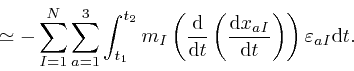
 , where
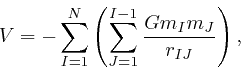
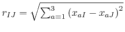 is
the distance between object
is
the distance between object
If
a quantity, such as the potential energy, depends on a number of quantities
![]() that can vary continuously, where
that can vary continuously, where ![]() represents the collection of those
quantities, and the index
represents the collection of those
quantities, and the index ![]() distinguishes the quantities in the collection,
and if the collection of data that gives the value of the dependent quantity
at each
distinguishes the quantities in the collection,
and if the collection of data that gives the value of the dependent quantity
at each ![]() , or in other words, at each set of values of the quantities
, or in other words, at each set of values of the quantities ![]() ,
is represented by a symbol
,
is represented by a symbol ![]() , then the collection of data that gives the
rate of change of the dependent quantity as the quantity
, then the collection of data that gives the
rate of change of the dependent quantity as the quantity ![]() changes, while
all the other quantities in
changes, while
all the other quantities in ![]() have fixed values, is usually represented as
have fixed values, is usually represented as
![]() , or alternatively as
, or alternatively as
![]() . The symbol
. The symbol ![]() is an alternative
notation for Leibniz's
is an alternative
notation for Leibniz's ![]() , and
, and
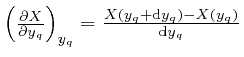 , where the quantities in the collection
 ![]() other than
other than ![]() all have the same values in both terms in the numerator in
the right-hand side as they have in the left-hand side, so their values don't
need to be displayed.
all have the same values in both terms in the numerator in
the right-hand side as they have in the left-hand side, so their values don't
need to be displayed.
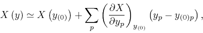
If the value
![]() changes smoothly with
changes smoothly with ![]() , or in other
words, smoothly with the quantities
, or in other
words, smoothly with the quantities ![]() in the collection
in the collection ![]() , then for
, then for ![]() near a reference collection
near a reference collection
![]() , in the sense that all the
quantities
, in the sense that all the
quantities
![]() are small in magnitude, the value
are small in magnitude, the value
![]() can be represented approximately as:
can be represented approximately as:
 , where
  for all
 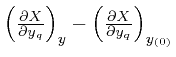 tend to 0 at least as fast as the
differences
tend to 0 at least as fast as the
differences
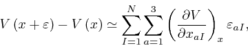
Applying
the above formula to the potential energy, with
![]() taken as
taken as ![]() , and
, and
![]() taken as
taken as ![]() ,
we have:
,
we have:
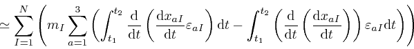
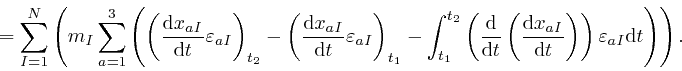
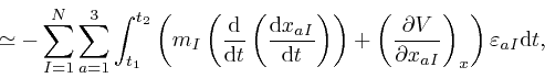
Combining this formula for the change of the potential energy with the formula
for the change of the kinetic energy we obtained
before it, we find that the
change to the action
 that
results from the replacement of
that
results from the replacement of ![]() by
by
![]() , is:
, is:
De Maupertuis's principle requires that the change to the action should tend
to 0 more rapidly than in proportion to ![]() , as
, as ![]() tends
to 0. But from the above formula, this is only possible for all
perturbations
tends
to 0. But from the above formula, this is only possible for all
perturbations ![]() such that
such that ![]() is 0 at
is 0 at ![]() and
and ![]() ,
and all the
,
and all the
![]() change smoothly with time, if:
change smoothly with time, if:
We are using Cartesian coordinates, so
![]() is the
is the ![]() 'th component of the velocity of the
'th component of the velocity of the ![]() 'th object, and
'th object, and
![]() , which is usually written as
, which is usually written as
 , is the
 ![]() 'th component of the acceleration of the
'th component of the acceleration of the
![]() 'th object. And by the definition of potential energy, the
'th object. And by the definition of potential energy, the ![]() 'th
component of the force on the
'th
component of the force on the ![]() 'th object is
'th object is
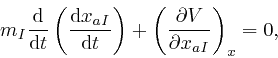
![]() . Thus the above equation is Newton's second law of motion.
. Thus the above equation is Newton's second law of motion.
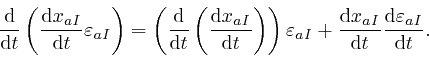
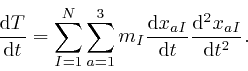
Let's now consider the rate of change with time of the total energy ![]() ,
when the objects move in accordance with Newton's second law of motion, which
we have just derived from de Maupertuis's principle. From Leibniz's rule for
the rate of change of a product, which we proved above,
the rate of change of
,
when the objects move in accordance with Newton's second law of motion, which
we have just derived from de Maupertuis's principle. From Leibniz's rule for
the rate of change of a product, which we proved above,
the rate of change of
 is
is
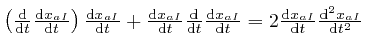 , so the rate of change with time
of the kinetic energy
, so the rate of change with time
of the kinetic energy ![]() is:
is:
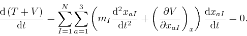
From
the sum of the above two formulae, we obtain the rate of change with time
of the total energy ![]() of the objects, when they move in accordance with
Newton's second law of motion, as:
of the objects, when they move in accordance with
Newton's second law of motion, as:
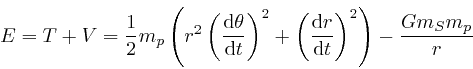
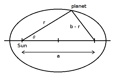
To illustrate the practical application of de Maupertuis's discovery, which is
sometimes called the principle of stationary action, let's consider a planet
in orbit around the Sun, neglecting the gravitational effects of the other
planets, which are relatively small. The mass ![]() of the Sun is much
greater than the mass
of the Sun is much
greater than the mass ![]() of the planet, so to a good approximation, we can
treat the Sun as fixed in position, and just consider the motion of the planet
around the Sun. The gravitational force on the planet is always in the
direction of the straight line from the planet to the Sun, so the planet stays
in the 2-dimensional plane defined by the straight line from the planet's
initial position to the Sun, and the direction of the planet's initial
velocity, which I shall assume is not exactly along that line.
of the planet, so to a good approximation, we can
treat the Sun as fixed in position, and just consider the motion of the planet
around the Sun. The gravitational force on the planet is always in the
direction of the straight line from the planet to the Sun, so the planet stays
in the 2-dimensional plane defined by the straight line from the planet's
initial position to the Sun, and the direction of the planet's initial
velocity, which I shall assume is not exactly along that line.
It is convenient to specify the planet's position in this plane by the
distance ![]() from the planet to the Sun, and the angle between the straight
line from the planet to the Sun, and the initial direction of that line. I
shall represent that angle by
from the planet to the Sun, and the angle between the straight
line from the planet to the Sun, and the initial direction of that line. I
shall represent that angle by ![]() , which is the Greek letter theta. To
keep the formulae as simple as possible, the angle
, which is the Greek letter theta. To
keep the formulae as simple as possible, the angle ![]() will be measured
not in degrees but in "radians", where 1 radian is the angle turned through
when something moving along a circular path has travelled a distance along the
circle equal to the radius of the circle. Thus a full
will be measured
not in degrees but in "radians", where 1 radian is the angle turned through
when something moving along a circular path has travelled a distance along the
circle equal to the radius of the circle. Thus a full ![]() rotation
is
rotation
is
![]() radians, and 1 radian is approximately
radians, and 1 radian is approximately
![]() .
.
Due to measuring the angle ![]() in radians, the distance travelled by the
planet when
in radians, the distance travelled by the
planet when ![]() increases by a small amount
increases by a small amount
![]() at fixed
at fixed
![]() is
is
![]() , and in the limit when
, and in the limit when
![]() tends
to 0, this is in the direction perpendicular to the straight line from the
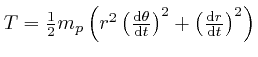
planet to the Sun. Thus the square of the planet's speed can be calculated
from
tends
to 0, this is in the direction perpendicular to the straight line from the
planet to the Sun. Thus the square of the planet's speed can be calculated
from
![]() and
and
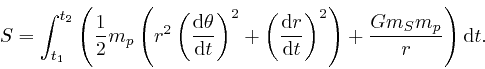
![]() using Pythagoras, so the kinetic energy of the planet is
using Pythagoras, so the kinetic energy of the planet is
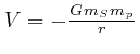
 . The
gravitational potential energy is
. The
gravitational potential energy is
 , so the action
is:
, so the action
is:
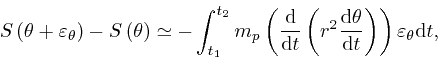
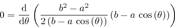
De
Maupertuis's principle requires that the change to the action should tend
to 0 more rapidly than in proportion to
![]() , as
, as
![]() tends to 0. But from the above formula, this is only
possible for all perturbations
tends to 0. But from the above formula, this is only
possible for all perturbations
![]() such that
such that
![]() is 0 at
is 0 at ![]() and
and ![]() , and
, and
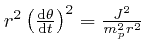
![]() changes smoothly with time, if
changes smoothly with time, if
![]() , for all relevant values
of
, for all relevant values
of ![]() . This means that
. This means that
![]() is
independent of time.
is
independent of time.
For a tiny amount of time ![]() , the area swept out by the straight
line from the Sun to the planet during the time interval
, the area swept out by the straight
line from the Sun to the planet during the time interval ![]() is
approximately
is
approximately
![]() , which is the area of the right-angled triangle made by the
straight lines from the Sun to the planet at the times
, which is the area of the right-angled triangle made by the
straight lines from the Sun to the planet at the times ![]() and
and
![]() , together with the straight line tangential to the circle of radius
, together with the straight line tangential to the circle of radius ![]() centred at the Sun, that meets that circle at the position of the planet at
time
centred at the Sun, that meets that circle at the position of the planet at
time ![]() . The difference between
. The difference between
![]() , and the area swept out by the straight
line from the Sun to the planet during the time interval
, and the area swept out by the straight
line from the Sun to the planet during the time interval ![]() , tends
to 0 in proportion to
, tends
to 0 in proportion to
![]() as
as ![]() tends
to 0, and thus more rapidly than in proportion to
tends
to 0, and thus more rapidly than in proportion to ![]() , so the rate
at which the straight line from the Sun to the planet sweeps out area is
, so the rate
at which the straight line from the Sun to the planet sweeps out area is
![]() . We found above
from de Maupertuis's principle that this is independent of time, so the
straight line from the Sun to the planet sweeps out equal areas in equal
times. This is the second of the three laws of planetary motion, which
Johannes Kepler
discovered by studying the astronomical measurements made by
Tycho Brahe.
. We found above
from de Maupertuis's principle that this is independent of time, so the
straight line from the Sun to the planet sweeps out equal areas in equal
times. This is the second of the three laws of planetary motion, which
Johannes Kepler
discovered by studying the astronomical measurements made by
Tycho Brahe.
The product
![]() , which is also
independent of time since the planet's mass
, which is also
independent of time since the planet's mass ![]() is constant, is called the
orbital angular momentum of the planet. I shall represent it by
is constant, is called the
orbital angular momentum of the planet. I shall represent it by ![]() . The
value of
. The
value of ![]() , like the value
, like the value ![]() of the planet's total energy, partly
characterizes the orbit of the planet.
of the planet's total energy, partly
characterizes the orbit of the planet.
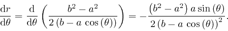
To find the possible shapes of the planet's orbit, we can convert the rate of
change of ![]() with time to the rate of change of
with time to the rate of change of ![]() with
with ![]() , using the
relation
, using the
relation
![]() . The time
interval during which
. The time
interval during which ![]() changes by a tiny amount
changes by a tiny amount
![]() is
is
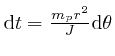 , so
, so
![]() .
Using this result and also the relation
.
Using this result and also the relation
 in the above formula
for the planet's total energy
in the above formula
for the planet's total energy ![]() , we find:
, we find:
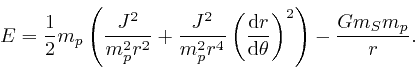
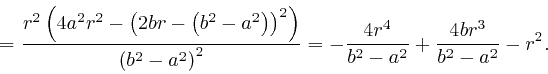
Rearranging this formula, we find:
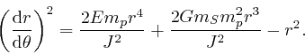
To use this formula to find the possible orbits of the planet, it is helpful
to know about the Cartesian coordinates of something moving around a circle,
and their rate of change with angle. If
something is moving along a circular
path, and ![]() is the angle in radians,
as above, between the straight line from
the centre of the moving object to the centre of the circle, and a fixed
straight line in the plane of the circle though the centre of the circle, then
the traditional names for the Cartesian coordinates of the centre of the
moving object, relative to the centre of the circle, in units of the radius of
the circle, are
is the angle in radians,
as above, between the straight line from
the centre of the moving object to the centre of the circle, and a fixed
straight line in the plane of the circle though the centre of the circle, then
the traditional names for the Cartesian coordinates of the centre of the
moving object, relative to the centre of the circle, in units of the radius of
the circle, are
![]() for the coordinate
parallel to the fixed straight line, and
for the coordinate
parallel to the fixed straight line, and
![]() for the coordinate perpendicular to the fixed straight line in the plane of
the circle. The directions of the coordinates are chosen so that
for the coordinate perpendicular to the fixed straight line in the plane of
the circle. The directions of the coordinates are chosen so that
![]() and
and
![]() . From Pythagoras, we have
. From Pythagoras, we have
![]() ,
for all
,
for all ![]() .
.
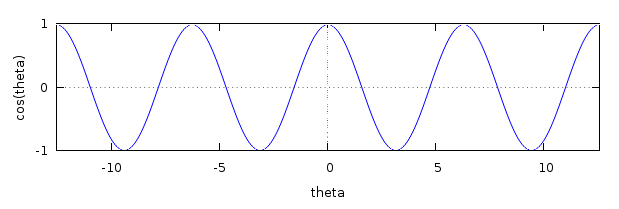
If the object starts at angle ![]() and goes round the circle
and goes round the circle ![]() times, so
that
times, so
that ![]() increases by
increases by ![]() , where
, where ![]() is any whole number, then the
Cartesian coordinates of the centre of the object come back to their initial
values, so that
is any whole number, then the
Cartesian coordinates of the centre of the object come back to their initial
values, so that
![]() , and
, and
![]() , for all whole numbers
, for all whole numbers ![]() . This
diagram shows
. This
diagram shows
![]() , for
, for ![]() in the range
in the range
![]() to
to ![]() .
.
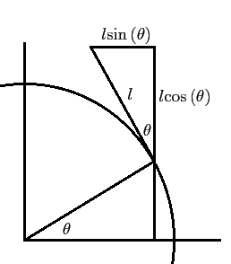
When the angle ![]() increases by a tiny amount
increases by a tiny amount
![]() , the
changes to the coordinates of the centre of the object are approximately the
same as they would be if the object moved a distance
, the
changes to the coordinates of the centre of the object are approximately the
same as they would be if the object moved a distance
![]() along the straight line tangential to the circle at
along the straight line tangential to the circle at ![]() instead of
exactly along the circle, where
instead of
exactly along the circle, where ![]() is the radius of the circle, and the
relative error of this approximation tends to 0 as
is the radius of the circle, and the
relative error of this approximation tends to 0 as
![]() tends
to 0. And from this diagram, the change to the Cartesian coordinate parallel
to the fixed straight line, when the centre of the object moves a distance
tends
to 0. And from this diagram, the change to the Cartesian coordinate parallel
to the fixed straight line, when the centre of the object moves a distance ![]() along the tangential straight line in the direction of increasing
along the tangential straight line in the direction of increasing ![]() , is
, is
![]() , and the change to the Cartesian
coordinate perpendicular to the fixed straight line is
, and the change to the Cartesian
coordinate perpendicular to the fixed straight line is
![]() . Thus:
. Thus:


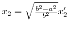
 Returning to the planet in orbit around the Sun, we can now confirm that the
above formula for
Returning to the planet in orbit around the Sun, we can now confirm that the
above formula for
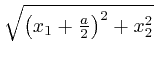
 implies that the orbit of the planet is an ellipse with the Sun at one focus,
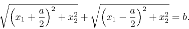
in agreement with Kepler's first law of planetary motion. An ellipse is the
curve formed by all the points in a plane such that the sum of the distances
from a point on the ellipse to two fixed points, called the focuses of the
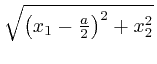
ellipse, has a fixed value. With the Sun at one focus, the distance from the
planet to that focus is
implies that the orbit of the planet is an ellipse with the Sun at one focus,
in agreement with Kepler's first law of planetary motion. An ellipse is the
curve formed by all the points in a plane such that the sum of the distances
from a point on the ellipse to two fixed points, called the focuses of the
ellipse, has a fixed value. With the Sun at one focus, the distance from the
planet to that focus is Rearranging this formula, we find:
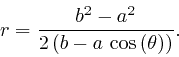
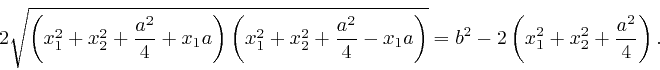
 is constant, so its rate of change is 0. Thus:


 for the planet's
orbit that we obtained above from de Maupertuis's
principle, we square both sides of the ellipse formula, and then use the
above
relation between
for the planet's
orbit that we obtained above from de Maupertuis's
principle, we square both sides of the ellipse formula, and then use the
above
relation between 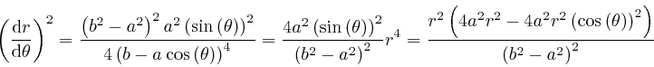
This exactly matches the formula for
for the
planet's orbit that we obtained above from de
Maupertuis's principle, if
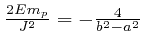 and
and
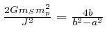 , so that
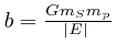 , and
, and
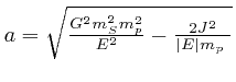 , where
![]() denotes the absolute value of
denotes the absolute value of ![]() . The value of
. The value of ![]() is negative because the planet is gravitationally bound to the Sun.
is negative because the planet is gravitationally bound to the Sun.
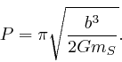
The time taken for the planet to complete one orbit is called the orbital
period, and I shall represent it by ![]() . We found above
that the rate at
which the straight line from the Sun to the planet sweeps out area is
. We found above
that the rate at
which the straight line from the Sun to the planet sweeps out area is
![]() . Thus
. Thus
 and
and
 by Pythagoras, so the
equation of the ellipse is:
by Pythagoras, so the
equation of the ellipse is:
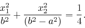
 , it becomes the equation of a circle
of radius
, it becomes the equation of a circle
of radius 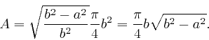 , so:
, so:
One of the clues that led to the discovery of Dirac-Feynman-Berezin sums came from the attempted application to electromagnetic radiation of discoveries about heat and temperature. In the next post in this series, Multiple Molecules, we'll look at some of those discoveries.
The software on this website is licensed for use under the Free Software Foundation General Public License.
Page last updated 4 May 2023. Copyright (c) Chris Austin 1997 - 2023. Privacy policy