 , is called the natural logarithm of
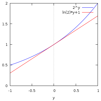
| Home | Blog index | Previous | Next | About | Privacy policy |
By Chris Austin. 27 November 2020.
An earlier version of this post was published on another website on 7 August 2012.
This is the second in a series of posts about the foundation of our understanding of the way the physical world works, which I am calling Dirac-Feynman-Berezin sums. The first post in the series is Action.
As in the previous post, I'll show you some formulae and things like that along the way, but I'll try to explain what all the parts mean as we go along, if we've not met them already, so you don't need to know about that sort of thing in advance.
One of the clues that led to the discovery of Dirac-Feynman-Berezin sums came from the attempted application to electromagnetic radiation of discoveries about heat and temperature. Today I would like to tell you about some of those discoveries.
Around 60 BC, Titus Lucretius Carus suggested in an epic poem, "On the Nature of Things," that matter consists of indivisible atoms moving incessantly in an otherwise empty void. In 1738 Daniel Bernoulli proposed that the pressure and temperature of gases are consequences of the random motions of large numbers of molecules. The theory was not immediately accepted, but around the middle of the nineteenth century, John James Waterston, August Krönig, Rudolf Clausius, and James Clerk Maxwell discovered that the everyday observations that things tend to have a temperature that can increase or decrease, and that the temperatures of adjacent objects tend to change towards a common intermediate value, follow from the random behaviour of large numbers of microscopic objects subject to Newton's laws, in particular the conservation of total energy.
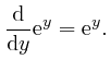
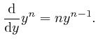
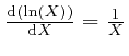
To understand how this happens, it is helpful to know about the rate of change
with ![]() of an expression such as
of an expression such as ![]() , which means
, which means ![]() to the power
to the power ![]() ,
where
,
where ![]() is a fixed number greater than 0, and
is a fixed number greater than 0, and ![]() could for example be time
or a position coordinate, measured in units of a fixed amount of time or a
fixed distance.
could for example be time
or a position coordinate, measured in units of a fixed amount of time or a
fixed distance. ![]() does not have to be a whole number, since any number
does not have to be a whole number, since any number ![]() can be approximated as accurately as desired by a ratio of the form
can be approximated as accurately as desired by a ratio of the form
![]() , where
, where ![]() and
and ![]() are whole numbers, and
are whole numbers, and
![]() is
the
is
the ![]() 'th power of the
'th power of the ![]() 'th root of
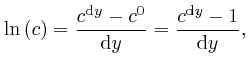
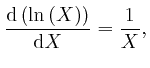
'th root of ![]() . The rate of change with
. The rate of change with ![]() of
of
![]() at
at ![]() , which we can write as
, is called the natural logarithm of
, which we can write as
, is called the natural logarithm of ![]() , and usually written
as
, and usually written
as
![]() . It was studied in the sixteenth century
by John Napier. I explained the meaning of an expression like
. It was studied in the sixteenth century
by John Napier. I explained the meaning of an expression like
![]() in the previous post, here.
in the previous post, here.
For example, this diagram shows ![]() in blue, for
in blue, for ![]() in the range
in the range ![]() to
1. The red line is the straight line with the same rate of change with
to
1. The red line is the straight line with the same rate of change with ![]() as
as ![]() at
at ![]() , and from its value
, and from its value
![]() at
at ![]() , we can read
from the graph that
, we can read
from the graph that
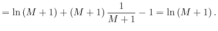
![]() . The symbol
. The symbol ![]() means, "approximately equal to."
means, "approximately equal to."
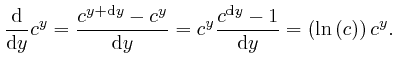
We have:
We now find:
The number
![]() such that
such that
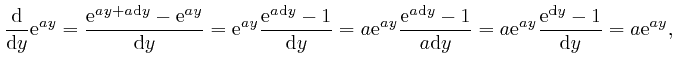
![]() is sometimes called Napier's number. From the above formula, we have:
is sometimes called Napier's number. From the above formula, we have:
For any fixed number ![]() , we have:
, we have:
 as the tiny quantity
 as the tiny quantity
From the above equation with ![]() chosen to be
chosen to be
![]() ,
we find that
,
we find that
for all ![]() , because both these expressions are equal to 1 for
, because both these expressions are equal to 1 for ![]() , and
they both satisfy the equation
, and
they both satisfy the equation
![]() . This equation fixes
. This equation fixes
![]() for all
for all ![]() once
once
![]() is given, because
is given, because
![]() can be calculated from
can be calculated from
![]() as accurately as desired,
by dividing up the interval from 0 to
as accurately as desired,
by dividing up the interval from 0 to ![]() into a great number of sufficiently
tiny intervals, and calculating the approximate value of
into a great number of sufficiently
tiny intervals, and calculating the approximate value of
![]() at the end of each tiny interval from its approximate value at the start of
that interval, by using
at the end of each tiny interval from its approximate value at the start of
that interval, by using
 .
.
From the above equation at ![]() , we find that
, we find that
for every number ![]() greater than 0. Thus for any numbers
greater than 0. Thus for any numbers ![]() and
and ![]() , both
greater than 0, we have
, both
greater than 0, we have
![]() . Thus:
. Thus:
If
![]() , so that the symbol
, so that the symbol ![]() , like the expression
, like the expression
![]() , represents the collection of data that gives the value of the
, represents the collection of data that gives the value of the
![]() -dependent quantity
-dependent quantity
![]() at each value of
at each value of ![]() , then from this
formula above, we have
, then from this
formula above, we have
![]() , and from this
formula above, we have
, and from this
formula above, we have
![]() , for all values of
, for all values of
![]() greater than 0. Thus
greater than 0. Thus
![]() , for all
, for all ![]() greater than 0, so:
greater than 0, so:
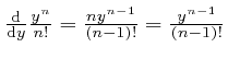
To calculate the value of Napier's number
![]() , we observe first that
for all positive whole numbers
, we observe first that
for all positive whole numbers ![]() :
:
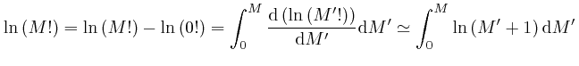
Therefore:
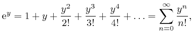
where ![]() is defined to be 1, and for each positive whole number
is defined to be 1, and for each positive whole number ![]() ,
, ![]() is
defined to be the product of all the whole numbers from 1 to
is
defined to be the product of all the whole numbers from 1 to ![]() . The
exclamation mark
. The
exclamation mark ![]() is usually read as "factorial". The
is usually read as "factorial". The ![]() mean
that the sum continues in accordance with the pattern shown by the terms
before the
mean
that the sum continues in accordance with the pattern shown by the terms
before the ![]() . The symbol
. The symbol ![]() is the Greek letter Sigma, and is
called the summation sign. I explained its meaning in the previous
post, here. The symbol
is the Greek letter Sigma, and is
called the summation sign. I explained its meaning in the previous
post, here. The symbol
![]() above the
above the ![]() , which is read as
"infinity", means that the sum is unending.
, which is read as
"infinity", means that the sum is unending.
The reason the above formula for
![]() is true is that the sum in the
right-hand side of the formula is equal to 1 for
is true is that the sum in the
right-hand side of the formula is equal to 1 for ![]() , and it satisfies the
same equation
, and it satisfies the
same equation
![]() as
as
![]() does.
So for the same reason as we discussed above, the sum in the right-hand side
of the formula is equal to
does.
So for the same reason as we discussed above, the sum in the right-hand side
of the formula is equal to ![]() , for all
, for all ![]() . The reason the expression
. The reason the expression
 satisfies
the equation
satisfies
the equation
![]() is that
is that
![]() on the first term in
on the first term in ![]() gives 0, and
gives 0, and
![]() on each term in
on each term in ![]() after the first gives
the preceding term in
after the first gives
the preceding term in ![]() , since from our observation above,
, since from our observation above,
 .
.
This argument that the expression
satisfies the equation
![]() assumes that the endless sum tends to a finite limiting
value as more and more terms are added, no matter how large the magnitude
assumes that the endless sum tends to a finite limiting
value as more and more terms are added, no matter how large the magnitude
![]() of
of ![]() is. In fact, the expression
is. In fact, the expression
![]() increases in magnitude with increasing
increases in magnitude with increasing ![]() for
for
![]() , and
then starts decreasing in magnitude more and more rapidly with increasing
, and
then starts decreasing in magnitude more and more rapidly with increasing ![]() ,
so that the endless sum always does tend to a finite limiting value, no matter
how large
,
so that the endless sum always does tend to a finite limiting value, no matter
how large
![]() is. If
is. If ![]() is larger than
is larger than
![]() ,
then the endless sum of all the terms from
,
then the endless sum of all the terms from
![]() onwards does not
exceed
onwards does not
exceed
 in magnitude.
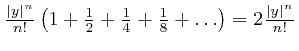
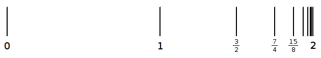
The endless sum
in magnitude.
The endless sum
![]() approaches 2 when it is continued without end, because each successive term
halves the difference between 2 and the sum of the terms up to that point, as
shown in this diagram.
approaches 2 when it is continued without end, because each successive term
halves the difference between 2 and the sum of the terms up to that point, as
shown in this diagram.
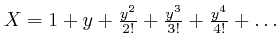
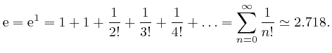
The above formula expressing
![]() as a sum of powers of
as a sum of powers of ![]() is an
example of a "Taylor series," named after Brook Taylor. For
is an
example of a "Taylor series," named after Brook Taylor. For ![]() , it
gives:
, it
gives:
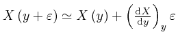
Let's now consider again, as in the previous post, here, the example of a collection of objects, such that
each object behaves approximately as though its mass is concentrated at a
single point, the objects are moving slowly compared to the speed of light,
and the forces between the objects arise from their potential energy ![]() ,
which depends on their positions but not on their motions. We'll continue to
assume that their motions are governed by Newton's laws, and thus by de
Maupertuis's principle of stationary action, which I explained in the previous post, here, and we'll now assume that the
objects are microscopic and their number is very large, so they could be atoms
in solids, liquids, gases, or living things. We'll use the same notation as
in the previous post, here.
,
which depends on their positions but not on their motions. We'll continue to
assume that their motions are governed by Newton's laws, and thus by de
Maupertuis's principle of stationary action, which I explained in the previous post, here, and we'll now assume that the
objects are microscopic and their number is very large, so they could be atoms
in solids, liquids, gases, or living things. We'll use the same notation as
in the previous post, here.
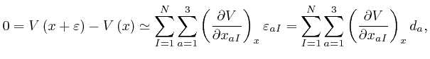
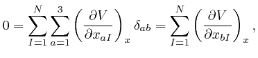
We'll use Cartesian coordinates for the positions of the objects, as we did
when we derived Newton's second law of motion from de Maupertuis's principle, in the previous post, here,
and we'll now assume that the potential energy ![]() depends only on the
relative positions of the objects, as in the example of the gravitational
potential energy, so that the value of
depends only on the
relative positions of the objects, as in the example of the gravitational
potential energy, so that the value of ![]() is unaltered if the positions
is unaltered if the positions ![]() of the objects are shifted by a common displacement
of the objects are shifted by a common displacement ![]() , so that
, so that
![]() , for all
, for all
![]() ,
,
![]() . The symbol
. The symbol ![]() means "less than or equal to."
means "less than or equal to."
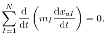
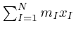
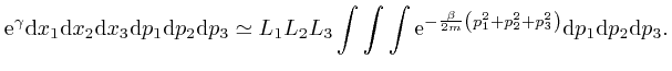
By adding up Newton's second law of motion for the ![]() objects, which we obtained from de Maupertuis's principle in the previous post, here, we find:
objects, which we obtained from de Maupertuis's principle in the previous post, here, we find:
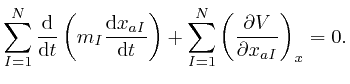
for all the relevant values 1, 2, and 3 of ![]() . Combining this result with
the formula we obtained above by adding up Newton's law of motion for the
. Combining this result with
the formula we obtained above by adding up Newton's law of motion for the ![]() objects, we find:
objects, we find:
The expression
![]() represents the velocity
of the
represents the velocity
of the ![]() 'th object, and the product of an object's mass and its velocity is
called its momentum. I shall let
'th object, and the product of an object's mass and its velocity is
called its momentum. I shall let ![]() represent the collection of data that
gives the momenta of all the objects at each moment in time, so that
represent the collection of data that
gives the momenta of all the objects at each moment in time, so that
![]() for all
for all
![]() ,
,
![]() , and times
, and times ![]() . The above result can then
be written:
. The above result can then
be written:

If the positions and momenta of all the objects are specified at one
particular time, then their values at every other time are determined by
Newton's second law of motion, which we obtained in the previous post,
here, from de Maupertuis's
principle. We'll now divide the range of the possible positions and momenta
of the objects into equal size "bins", and ask what the most likely number
of objects in each bin will be, if the objects are randomly distributed among
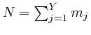
the bins, subject to the total energy of the objects having a fixed value ![]() .
.
We'll assume that each bin is sufficiently small that we can treat the
positions and momenta of objects in the same bin as approximately equal to one
another, but also sufficiently large that the number of objects in a typical
bin will be large. For this to be possible, we'll assume that the total
number of objects, ![]() , is very large. This is reasonable for things in the
everyday world, since the number of atoms in a kilogram of matter is in the
range from about
, is very large. This is reasonable for things in the
everyday world, since the number of atoms in a kilogram of matter is in the
range from about ![]() to
to ![]() .
.
We'll allow for the possibility that there could be a number of different
types of object, such that the masses and interactions of objects of the same
type are either identical or very similar to one another, so that the kinetic
energy ![]() and the potential energy
and the potential energy ![]() are either exactly or approximately
unaltered if the positions and momenta of two objects of the same type are
swapped. Objects of different types could be different types of atom, or
atoms of the same type in different situations. For example we'll treat two
oxygen atoms as different types of object if they form parts of gas molecules
contained in separate containers, or if one is part of a gas molecule and the
other is part of the wall of a glass container. We'll assume that the number
of objects of each different type is very large.
are either exactly or approximately
unaltered if the positions and momenta of two objects of the same type are
swapped. Objects of different types could be different types of atom, or
atoms of the same type in different situations. For example we'll treat two
oxygen atoms as different types of object if they form parts of gas molecules
contained in separate containers, or if one is part of a gas molecule and the
other is part of the wall of a glass container. We'll assume that the number
of objects of each different type is very large.
We'll assume that the total momentum of the objects is 0, so that the position
of their centre of mass
 is independent of time, and
we'll assume that if any of the objects are parts of liquid or gas molecules,
then some of the other objects form solid containers that prevent the liquids
or gases from spreading without limit. The number of relevant bins is
therefore finite, because the position coordinates of all the objects are
bounded, and the momenta of the objects are also bounded, because we assumed
above that the objects are moving slowly compared to the speed of light. We'll
denote the number of relevant bins by
is independent of time, and
we'll assume that if any of the objects are parts of liquid or gas molecules,
then some of the other objects form solid containers that prevent the liquids
or gases from spreading without limit. The number of relevant bins is
therefore finite, because the position coordinates of all the objects are
bounded, and the momenta of the objects are also bounded, because we assumed
above that the objects are moving slowly compared to the speed of light. We'll
denote the number of relevant bins by ![]() .
.
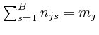
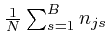
I shall let ![]() represent the collection of data that gives the total number
of objects of each type, so that if
represent the collection of data that gives the total number
of objects of each type, so that if ![]() represents one of the different types
of object, then
represents one of the different types
of object, then ![]() is the total number of objects of type
is the total number of objects of type ![]() , and I shall
let
, and I shall
let ![]() represent the collection of data that gives the number of objects of
each type in each of the bins into which the range of possible positions and
momenta of the objects has been divided, so that if
represent the collection of data that gives the number of objects of
each type in each of the bins into which the range of possible positions and
momenta of the objects has been divided, so that if ![]() represents one of the
bins, then
represents one of the
bins, then ![]() is the number of objects of type
is the number of objects of type ![]() in bin
in bin ![]() .
.
The objects can be distinguished from one another even if they are of the same
type and identical to one another, because we can trace their motions back to
a particular time, and "label" identical objects by the positions and
momenta they had at that time. The number of different assignments of the
![]() objects of type
objects of type ![]() to the bins is
to the bins is ![]() , because each of the
objects can be assigned independently to any of the
, because each of the
objects can be assigned independently to any of the ![]() bins, and of these
bins, and of these
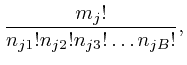
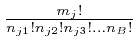
![]() assignments, the number such that
assignments, the number such that ![]() of the objects of type
of the objects of type
![]() are in bin 1,
are in bin 1, ![]() of them are in bin 2, and so on, is:
of them are in bin 2, and so on, is:
To understand why the above formula gives the number of different assignments
of the ![]() objects of type
objects of type ![]() to the
to the ![]() bins, such that for each whole
number
bins, such that for each whole
number ![]() in the range 1 to
in the range 1 to ![]() , the number of objects of type
, the number of objects of type ![]() in bin
in bin ![]() is
is ![]() , we note first that the number of different ways of putting
, we note first that the number of different ways of putting ![]() distinguishable objects in
distinguishable objects in ![]() distinguishable places, such that exactly one
object goes to each place, is
distinguishable places, such that exactly one
object goes to each place, is ![]() , because we can put the first object in any
of the
, because we can put the first object in any
of the ![]() places, the second object in any of the remaining
places, the second object in any of the remaining ![]() places,
and so on. So if there were
places,
and so on. So if there were ![]() distinguishable places in bin
distinguishable places in bin ![]() , for
each
, for
each ![]() in the range 1 to
in the range 1 to ![]() , then the number of different ways of putting
the
, then the number of different ways of putting
the ![]() objects in these
objects in these
![]() distinct places would be
distinct places would be ![]() . This overcounts the number of different
assignments of the objects to the bins by a factor
. This overcounts the number of different
assignments of the objects to the bins by a factor
![]() , because we can divide up the
, because we can divide up the ![]() arrangements into
classes, such that arrangements are in the same class if they only differ by
permuting objects within bins. Each class then corresponds to a different
assignment of the objects to the bins. The number of the
arrangements into
classes, such that arrangements are in the same class if they only differ by
permuting objects within bins. Each class then corresponds to a different
assignment of the objects to the bins. The number of the ![]() arrangements in each class is
arrangements in each class is
![]() , so
the number of different classes is
, so
the number of different classes is
 .
.
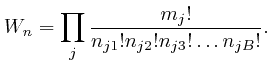
The number of different assignments of all ![]() objects to the
objects to the ![]() bins is
bins is
![]() , and of these, the number such that
, and of these, the number such that ![]() of the objects of type
of the objects of type ![]() are in bin
are in bin ![]() , for all
, for all ![]() and
and ![]() , which I shall denote by
, which I shall denote by ![]() , is the
product of the above number over
, is the
product of the above number over ![]() , which we can write as:
, which we can write as:
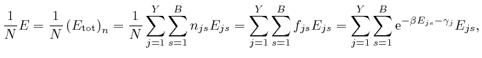
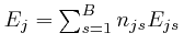
The total energy
![]() of the objects, when the numbers of objects of the different types
in the different bins are given by the collection of data
of the objects, when the numbers of objects of the different types
in the different bins are given by the collection of data ![]() , is
approximately:
, is
approximately:
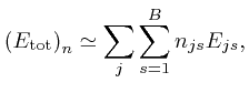
where ![]() is the energy of an object of type
is the energy of an object of type ![]() in the centre of bin
in the centre of bin
![]() . If we randomly drop the
. If we randomly drop the ![]() objects into the
objects into the ![]() bins, and discard the
result unless the total energy
bins, and discard the
result unless the total energy
![]() differs from
differs from ![]() by at
most a fixed small amount, then the probability that the numbers of objects of
the different types in the different bins are given by
by at
most a fixed small amount, then the probability that the numbers of objects of
the different types in the different bins are given by ![]() is
is ![]() , divided
by the sum of
, divided
by the sum of ![]() over all
over all ![]() such that
such that
![]() is close enough to
is close enough to
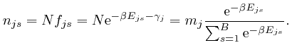
![]() . Thus if the objects are randomly distributed among the bins, subject to
the total energy of the objects having a fixed value
. Thus if the objects are randomly distributed among the bins, subject to
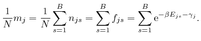
the total energy of the objects having a fixed value ![]() , then the most likely
number of objects of each type in each bin will be given by the distribution
, then the most likely
number of objects of each type in each bin will be given by the distribution
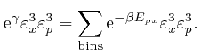
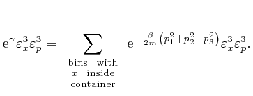
![]() for which
for which ![]() reaches its maximum value, among all the distributions
reaches its maximum value, among all the distributions
![]() for which
for which
![]() is approximately equal to
is approximately equal to ![]() .
.
To find the distribution ![]() for which
for which ![]() reaches its maximum value,
subject to
reaches its maximum value,
subject to
![]() , we'll use the observation that the slope of a smooth hill is zero
at the top of the hill. Thus we'll look for the distribution
, we'll use the observation that the slope of a smooth hill is zero
at the top of the hill. Thus we'll look for the distribution ![]() such that
the rate of change of
such that
the rate of change of ![]() with each of the numbers
with each of the numbers ![]() would be 0, if
it were not for the requirement that
would be 0, if
it were not for the requirement that
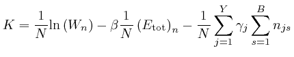
![]() . For
convenience we'll do the calculation for
. For
convenience we'll do the calculation for
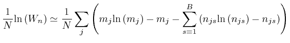
![]() rather than for
rather than for ![]() , so that the product of factors in
, so that the product of factors in ![]() becomes the sum
of the natural logarithms of those factors, due to the result we found above.
This will give the same result for the most likely distribution
becomes the sum
of the natural logarithms of those factors, due to the result we found above.
This will give the same result for the most likely distribution ![]() , because
, because
![]() increases with increasing
increases with increasing ![]() for all
for all
![]() greater than 0, due to the result we found above, so that the
greater than 0, due to the result we found above, so that the ![]() that
gives the largest value of
that
gives the largest value of ![]() will also be the
will also be the ![]() that gives the largest
value of
that gives the largest
value of
![]() .
.
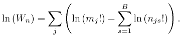
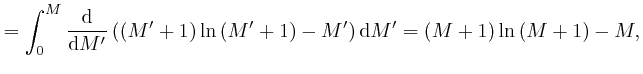
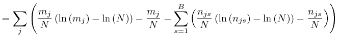
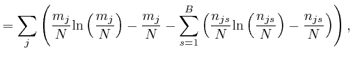
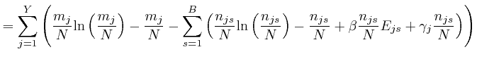
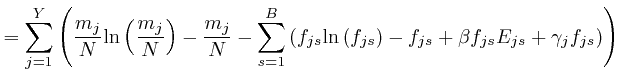
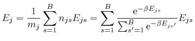
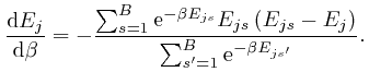
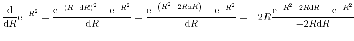
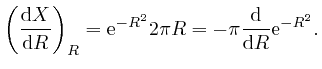
From the formula above for ![]() , we have:
, we have:
For very large ![]() , we can therefore write:
, we can therefore write:

 , for all
 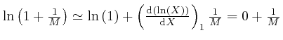 , so the error of the above
approximation decreases in proportion to
, so the error of the above
approximation decreases in proportion to
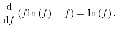
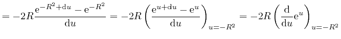
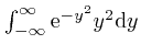
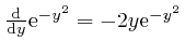
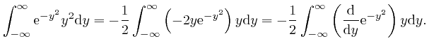
And from
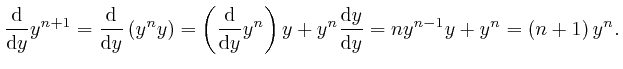
together with Leibniz's rule for the
rate of change of a product, which we obtained in the previous post,
here, we have:

since from above,
![]() and from above,
and from above,
![]() . The above approximation for
. The above approximation for
![]() is in error by an amount that increases slowly for large
is in error by an amount that increases slowly for large ![]() , but its relative
error tends to 0 for large
, but its relative
error tends to 0 for large ![]() , so it is accurate enough to use for finding
the distribution
, so it is accurate enough to use for finding
the distribution ![]() for which
for which ![]() reaches its maximum value, since the
numbers
reaches its maximum value, since the
numbers ![]() will all increase in proportion to the total number of
objects
will all increase in proportion to the total number of
objects ![]() , which we have assumed to be very large. We can also use the
simpler approximation:
, which we have assumed to be very large. We can also use the
simpler approximation:
Thus we have:
 , for each type of object
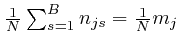
It is convenient to think of the ratios
![]() as coordinates in
a "space", which I shall call the space of bin fractions, since
as coordinates in
a "space", which I shall call the space of bin fractions, since
![]() is the fraction of the total number of objects
is the fraction of the total number of objects ![]() which are objects
of type
which are objects
of type ![]() in bin
in bin ![]() . The numbers
. The numbers ![]() are restricted to be whole
numbers, but for fixed values of the ratios
are restricted to be whole
numbers, but for fixed values of the ratios
![]() , these numbers
will be proportional to
, these numbers
will be proportional to ![]() , which we have assumed is very large. Thus the
ratios
, which we have assumed is very large. Thus the
ratios
![]() only change by tiny amounts when
only change by tiny amounts when ![]() change
by
change
by ![]() , where the symbol
, where the symbol ![]() means "plus or minus," so since
means "plus or minus," so since
![]() depends smoothly on
depends smoothly on ![]() for all numbers
for all numbers ![]() , we can think of the coordinates
, we can think of the coordinates
![]() as effectively
continuous. If the number of types of object is
as effectively
continuous. If the number of types of object is ![]() , then the space of bin
fractions has
, then the space of bin
fractions has ![]() dimensions, since a point in this space is specified by the
dimensions, since a point in this space is specified by the
![]() numbers
numbers
![]() .
.
The equation
![]() imposes one relation among the
imposes one relation among the ![]() coordinates of the space of bin
fractions, so it defines a
coordinates of the space of bin
fractions, so it defines a
![]() -dimensional "surface" in
this space. We are looking for the point
-dimensional "surface" in
this space. We are looking for the point ![]() on this surface at which
on this surface at which
![]() reaches the largest value it takes anywhere
on this surface. If we think of
reaches the largest value it takes anywhere
on this surface. If we think of
![]() as the
height of a smooth "hill", then since the slope of a smooth hill is 0 in
each direction at the top of the hill, the rate of change of
as the
height of a smooth "hill", then since the slope of a smooth hill is 0 in
each direction at the top of the hill, the rate of change of
![]() is 0 in each direction along the surface, at the point
is 0 in each direction along the surface, at the point ![]() on the surface where
on the surface where
![]() reaches its maximum
value. However the rate of change of
reaches its maximum
value. However the rate of change of
![]() in
directions that are not along the surface does not have to be 0 at that point.
So we are looking for a point
in
directions that are not along the surface does not have to be 0 at that point.
So we are looking for a point ![]() on the surface such that the rate of
change
on the surface such that the rate of
change
![]() in every direction, whether along the
surface or not, is a multiple of the rate of change of
in every direction, whether along the
surface or not, is a multiple of the rate of change of
![]() in that direction,
since the rate of change of
in that direction,
since the rate of change of
![]() along the surface is
0.
along the surface is
0.
We can do that by looking for a point ![]() for which an expression
for which an expression
The ![]() equations
, one for each type of object
equations
, one for each type of object
![]() , similarly each define a
, similarly each define a
![]() -dimensional surface in
the space of bin fractions, and we'll take these equations into account by
using
-dimensional surface in
the space of bin fractions, and we'll take these equations into account by
using ![]() additional Lagrange multipliers
additional Lagrange multipliers ![]() , one for each of these
equations, where
, one for each of these
equations, where ![]() is the Greek letter gamma. So we'll look for a
point
is the Greek letter gamma. So we'll look for a
point ![]() in the space of bin fractions for which an expression:
in the space of bin fractions for which an expression:
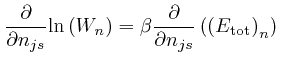
If this is 0 for all ![]() and all
and all ![]() at a point
at a point ![]() in the space of bin
fractions, then the rate of change of
in the space of bin
fractions, then the rate of change of ![]() will be 0 in any direction where the
rates of change of
will be 0 in any direction where the
rates of change of
![]() and all the quantities
and all the quantities
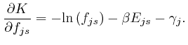
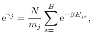
 are 0. From the
result we found above, this expression for
are 0. From the
result we found above, this expression for
![]() is 0 when:
is 0 when:
And when the value of each ![]() is given by the above formula, the rate
of change of
is given by the above formula, the rate
of change of
![]() , in any direction
in the space of bin fractions, is
, in any direction
in the space of bin fractions, is ![]() times the rate of change of
times the rate of change of
![]() in
that direction, plus the sum, over the object types
in
that direction, plus the sum, over the object types ![]() , of
, of ![]() times
the rate of change of
times
the rate of change of
 in that direction.
Remembering that ![]() and the
and the ![]() are fixed numbers whose values
will be chosen later, we'll now define the value of
are fixed numbers whose values
will be chosen later, we'll now define the value of
![]() , and the
numbers
, and the
numbers
![]() , to be such that the equation
, to be such that the equation
![]() , and
the
, and
the ![]() equations
equations
 , are
all satisfied at the point where the value of each
, are
all satisfied at the point where the value of each
![]() is given by the above formula.
is given by the above formula.
For fixed values of
![]() , and the numbers
, and the numbers
![]() , each
of these
, each
of these ![]() equations defines a
equations defines a
![]() -dimensional
surface in the space of bin fractions, and the intersection of these
-dimensional
surface in the space of bin fractions, and the intersection of these ![]() surfaces defines a
surfaces defines a
![]() -dimensional "surface" in the
space of bin fractions. This
-dimensional "surface" in the
space of bin fractions. This
![]() -dimensional surface
is the surface on which the
-dimensional surface
is the surface on which the ![]() equations
equations
![]() and
are all satisfied, so
in any direction tangential to this
and
are all satisfied, so
in any direction tangential to this
![]() -dimensional
surface, the rates of change of
-dimensional
surface, the rates of change of
![]() and
are all 0. Thus at the point on this
and
are all 0. Thus at the point on this
![]() -dimensional surface where the value of each
-dimensional surface where the value of each ![]() is given by
the above formula, the rate of change of
is given by
the above formula, the rate of change of
![]() , in any direction tangential to this
, in any direction tangential to this
![]() -dimensional surface, is 0.
-dimensional surface, is 0.
I'll refer to this
![]() -dimensional surface in the
space of bin fractions as
-dimensional surface in the
space of bin fractions as
![]() , since the fixed
values of
, since the fixed
values of
![]() and the numbers
and the numbers
![]() on it are
determined by the fixed values of
on it are
determined by the fixed values of ![]() and the
and the ![]() . Since the
maximum value of
. Since the
maximum value of ![]() in the region where all
in the region where all ![]() are
are ![]() is attained
when the value of each
is attained
when the value of each ![]() is given by the above formula, and the values
of
is given by the above formula, and the values
of
![]() and the
are all fixed on
and the
are all fixed on
![]() , the maximum value of
, the maximum value of
![]() on
on
![]() , in the region where all
, in the region where all ![]() are
are ![]() , is attained when the value of each
, is attained when the value of each ![]() is given by the
above formula.
is given by the
above formula.
From the formula for
![]() as above, the fixed
values of the
as above, the fixed
values of the ![]() quantities
quantities
![]() and the
and the
![]() are
determined in terms of the
are
determined in terms of the ![]() quantities
quantities ![]() and the
and the ![]() by
the formulae:
by
the formulae:
From the last formula above:
so from the formula above:
From above, Napier's number
![]() has the value
has the value
![]() , so if
, so if ![]() was negative, then for a given type of object
was negative, then for a given type of object ![]() ,
,
![]() would be larger for bins for which the energy
would be larger for bins for which the energy ![]() at their
centres is larger, and if
at their
centres is larger, and if ![]() was 0,
was 0, ![]() would be the same for all
bins, no matter how large the energy
would be the same for all
bins, no matter how large the energy ![]() at their centres. In either
of these cases, there would be no justification for our assumption that the
objects are all moving slowly compared to the speed of light, so I'll assume
that
at their centres. In either
of these cases, there would be no justification for our assumption that the
objects are all moving slowly compared to the speed of light, so I'll assume
that ![]() .
.
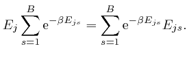
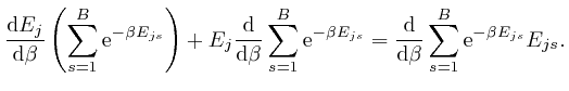
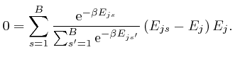
From the above formula for ![]() , we have:
, we have:
where:
We observe that ![]() is a weighted average of the energies
is a weighted average of the energies ![]() of the
objects of type
of the
objects of type ![]() at the bin centres, such that the relative weights of
larger
at the bin centres, such that the relative weights of
larger ![]() decrease as
decrease as ![]() increases, so we expect that
increases, so we expect that ![]() will
decrease as
will
decrease as ![]() increases. To check this, we note that by a
rearrangement of the above formula:
increases. To check this, we note that by a
rearrangement of the above formula:
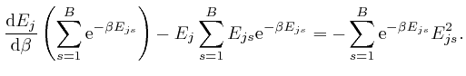
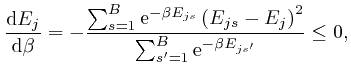
 , and shows that for finite
  unless
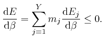
From the formula above for ![]() in terms of the
in terms of the ![]() , we have:
, we have:
If each different assignment of the
 objects to the
![]() bins, consistent with the given total energy
bins, consistent with the given total energy ![]() of the system, is equally
likely, then as we observed above, the most likely values of the numbers
of the system, is equally
likely, then as we observed above, the most likely values of the numbers ![]() will be those for which
will be those for which ![]() reaches its maximum value, consistent with
the given total energy
reaches its maximum value, consistent with
the given total energy ![]() . If the numbers
. If the numbers ![]() initially differ from
these values, then over the course of time, we expect them to tend towards
these values. The reason for this is that we have assumed that the total
energy can be expressed as a sum of the energies of the individual objects. There will be small corrections to this assumption, due for example to
interactions between gas molecules in the same container, or small mutual
interactions between atoms vibrating near the surfaces of different containers
that are touching one another. These interactions will occur randomly and
can change the numbers
initially differ from
these values, then over the course of time, we expect them to tend towards
these values. The reason for this is that we have assumed that the total
energy can be expressed as a sum of the energies of the individual objects. There will be small corrections to this assumption, due for example to
interactions between gas molecules in the same container, or small mutual
interactions between atoms vibrating near the surfaces of different containers
that are touching one another. These interactions will occur randomly and
can change the numbers
![]() by small amounts such as
by small amounts such as
![]() , so their net effect is that the numbers
, so their net effect is that the numbers ![]() will drift
towards their most likely values.
will drift
towards their most likely values.
It's convenient, now, to change the meaning of ![]() , which I defined above to be the average energy of an object of type
, which I defined above to be the average energy of an object of type ![]() , to be the total energy of the objects of type
, to be the total energy of the objects of type ![]() , instead.
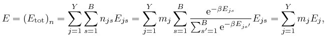
The total energy
, instead.
The total energy
 of the objects of type
![]() depends on the numbers
depends on the numbers ![]() , so a drift of these numbers with time
can result in a net transfer of energy from one type of object to another,
while the total energy remains constant. If two systems, each of which might
contain a number of different types of object, are initially separated from
one another, with total energies
, so a drift of these numbers with time
can result in a net transfer of energy from one type of object to another,
while the total energy remains constant. If two systems, each of which might
contain a number of different types of object, are initially separated from
one another, with total energies ![]() and
and ![]() and initial values
and initial values ![]() and
and ![]() of
of ![]() , and are brought into contact with one another, such
that neither system exerts any mechanical, electromagnetic, or gravitational
force on the other, but the numbers
, and are brought into contact with one another, such
that neither system exerts any mechanical, electromagnetic, or gravitational
force on the other, but the numbers ![]() for each system can drift due to
random microscopic interactions between parts of the two systems as above, for
example where containers of gas that were initially separated are now touching
one another, then the numbers
for each system can drift due to
random microscopic interactions between parts of the two systems as above, for
example where containers of gas that were initially separated are now touching
one another, then the numbers ![]() for each system will drift towards
values corresponding to a common final value
for each system will drift towards
values corresponding to a common final value ![]() of
of ![]() for both
systems, which is the value for which
for both
systems, which is the value for which ![]() for the combined system is
maximized, when the total energy of the combined system is
for the combined system is
maximized, when the total energy of the combined system is ![]() .
.
If the initial values ![]() and
and ![]() of
of ![]() are such that
are such that
![]() , then the final common value
, then the final common value ![]() of
of ![]() cannot be such that
cannot be such that
![]() , for by the result above, that would
mean that the final energies
, for by the result above, that would
mean that the final energies ![]() and
and ![]() of the two systems
satisfy
of the two systems
satisfy
![]() and
and
![]() , in contradiction with the
conservation of the total energy of the combined system, which we found above
follows from Newton's laws or de Maupertuis's principle, and which implies
that
, in contradiction with the
conservation of the total energy of the combined system, which we found above
follows from Newton's laws or de Maupertuis's principle, and which implies
that
![]() . And similarly,
. And similarly, ![]() cannot be
such that
cannot be
such that
![]() , for by the result above, that would imply
, for by the result above, that would imply
![]() and
and
![]() , which again contradicts the conservation of the
total energy of the combined system. Thus we must have
, which again contradicts the conservation of the
total energy of the combined system. Thus we must have
![]() , so if
, so if
![]() , then
, then
![]() .
.
If
![]() , and each of the two systems contains at least one type
of object for which
, and each of the two systems contains at least one type
of object for which ![]() has different values for at least two different
bins, then from the result above,
has different values for at least two different
bins, then from the result above,
![]() and
and
![]() , so
, so
![]() , and
, and
![]() and
and
![]() , so the drift of the
numbers
, so the drift of the
numbers ![]() to their final values results in a net transfer of energy
from the second system to the first. The values of
to their final values results in a net transfer of energy
from the second system to the first. The values of ![]() ,
, ![]() , and
, and
![]() are determined by the requirement that
are determined by the requirement that
![]() , so that
, so that
![]() .
.
These results show that ![]() has the basic observed properties of
temperature, except that
has the basic observed properties of
temperature, except that ![]() increases where temperature decreases, and
conversely. To determine the relation between
increases where temperature decreases, and
conversely. To determine the relation between ![]() and temperature, we'll
consider the example of an ideal gas, which is a collection of randomly moving
non-interacting molecules of mass
and temperature, we'll
consider the example of an ideal gas, which is a collection of randomly moving
non-interacting molecules of mass ![]() , enclosed in a container. In
accordance with our assumptions above, we'll assume that each molecule behaves
approximately as though its mass is concentrated at a single point.
, enclosed in a container. In
accordance with our assumptions above, we'll assume that each molecule behaves
approximately as though its mass is concentrated at a single point.
We'll take the container of the gas to be a box whose edges are aligned with
the Cartesian coordinate directions, such that the interior dimensions of the
box are ![]() ,
, ![]() , and
, and ![]() . The total momentum of the molecules and the
box is 0 in accordance with our assumption above, so the position of the
centre of mass of the molecules and the box is independent of time. The
molecules are moving randomly in the interior of the box, and we'll assume
that the box is sufficiently rigid, and its mass is sufficiently large
compared to the mass
. The total momentum of the molecules and the
box is 0 in accordance with our assumption above, so the position of the
centre of mass of the molecules and the box is independent of time. The
molecules are moving randomly in the interior of the box, and we'll assume
that the box is sufficiently rigid, and its mass is sufficiently large
compared to the mass ![]() of each molecule, that we can treat the box to a good
approximation as staying in a fixed position. The ranges of the position
coordinates in the interior of the box are
of each molecule, that we can treat the box to a good
approximation as staying in a fixed position. The ranges of the position
coordinates in the interior of the box are
![]() ,
,
![]() , and
, and
![]() . The potential energy
. The potential energy ![]() is 0 when all
the molecules are in the interior of the box, and
is 0 when all
the molecules are in the interior of the box, and ![]() when any of the
molecules is outside the interior of the box.
when any of the
molecules is outside the interior of the box.
We'll now divide the range of the possible positions and momenta of each
molecule into equal size bins as I described above, and we'll choose each bin
to be a box with its edges aligned with the Cartesian coordinate directions,
such that the length of each position edge of a bin is
![]() and the
difference between the values of a momentum coordinate at the ends of a
momentum edge of a bin is
and the
difference between the values of a momentum coordinate at the ends of a
momentum edge of a bin is
![]() . The sizes of the bin edges
. The sizes of the bin edges
![]() and
and
![]() are sufficiently small that we can treat
all the molecules in a bin as being approximately at the same position and
having approximately the same momentum, but sufficiently large that the number
of molecules in a bin is large. This is not a problem for gas containers of
everyday sizes, since the number of molecules in a cubic metre of air, to the
nearest power of 10, is about
are sufficiently small that we can treat
all the molecules in a bin as being approximately at the same position and
having approximately the same momentum, but sufficiently large that the number
of molecules in a bin is large. This is not a problem for gas containers of
everyday sizes, since the number of molecules in a cubic metre of air, to the
nearest power of 10, is about ![]() .
.
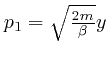
From above, the momentum ![]() of a molecule at position
of a molecule at position ![]() moving with speed
moving with speed
![]() is
is ![]() , so the kinetic energy of
the molecule is:
, so the kinetic energy of
the molecule is:
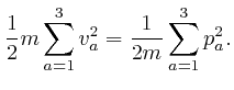
If ![]() is in the interior of the container, then the potential energy
is in the interior of the container, then the potential energy ![]() is
0, so from the formula above for the kinetic energy of a molecule:
is
0, so from the formula above for the kinetic energy of a molecule:
If we did the calculations in the limit where the sizes
![]() and
and
![]() of the bin edges tend to 0, this formula would be exact. We
assumed above that
of the bin edges tend to 0, this formula would be exact. We
assumed above that
![]() and
and
![]() are sufficiently small
that we can treat all the molecules in a bin as being approximately at the
same position and having approximately the same momentum, so I'll treat this
formula as exact. We therefore have:
are sufficiently small
that we can treat all the molecules in a bin as being approximately at the
same position and having approximately the same momentum, so I'll treat this
formula as exact. We therefore have:
 , so the value of
on the magnitudes
, so the value of
on the magnitudes
We'll complete the calculation of
![]() by first calculating
the number
by first calculating
the number
 , and
we'll calculate this number by first calculating its square, which I'll
represent by
, and
we'll calculate this number by first calculating its square, which I'll
represent by
![]() . We can write this as:
. We can write this as:
 is
is
 or higher
powers of
or higher
powers of
Thus:
since
![]() . Thus
. Thus
![]() , since the limit of
, since the limit of
![]() as
as ![]() tends to
tends to ![]() is 0. Thus:
is 0. Thus:
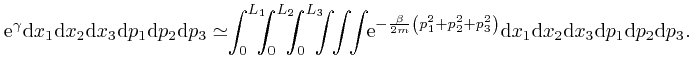
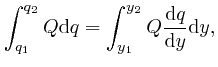
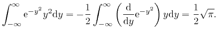
We now observe that according to the explanation I gave in the previous
post, here, of the meaning of the integral of a quantity, say ![]() , that
depends smoothly on another quantity, say
, that
depends smoothly on another quantity, say ![]() , over a range of values of
, over a range of values of ![]() ,
say from
,
say from ![]() to
to ![]() , where
, where
![]() , the range of
, the range of ![]() from
from ![]() to
to
![]() is divided up into a great number of tiny intervals, and the integral
is divided up into a great number of tiny intervals, and the integral
![]() is approximately the sum of a contribution
from each of these tiny intervals, such that the contribution from each tiny
interval is the value of
is approximately the sum of a contribution
from each of these tiny intervals, such that the contribution from each tiny
interval is the value of ![]() at some point in that tiny interval, times the
difference between the values of
at some point in that tiny interval, times the
difference between the values of ![]() at the ends of that tiny interval. The
exact value of the integral is the limit of sums of this form, as the tiny
intervals become so small and their number so great, that the size of the
largest tiny interval tends to 0. So if
at the ends of that tiny interval. The
exact value of the integral is the limit of sums of this form, as the tiny
intervals become so small and their number so great, that the size of the
largest tiny interval tends to 0. So if ![]() in turn depends on another
quantity, say
in turn depends on another
quantity, say ![]() , such that
, such that
![]() , the rate of
change of
, the rate of
change of ![]() with respect to
with respect to ![]() , is
, is ![]() for all values of
for all values of ![]() from
from ![]() to
to ![]() , then we have:
, then we have:
 , and the error of this approximation tends to 0 more rapidly than
in proportion to
, and the error of this approximation tends to 0 more rapidly than
in proportion to
From this observation, with ![]() taken as
taken as
![]() ,
, ![]() taken as
taken as ![]() , and
, and ![]() taken as
taken as
 ,
so that
,
so that
 ,
,
 , and
, and
 , we find from
the result above that:
, we find from
the result above that:
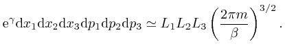
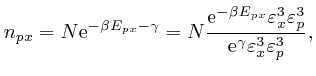
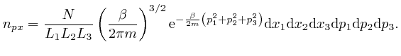
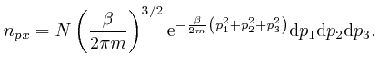
So from the formula above, the most likely number of molecules in a bin
centred at a position ![]() inside the container and momentum
inside the container and momentum ![]() , with edge
sizes
, with edge
sizes
![]() ,
,
![]() ,
,
![]() ,
,
![]() ,
,
![]() , and
, and
![]() , is:
, is:
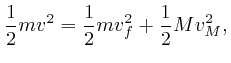
When an object of mass ![]() moving with velocity
moving with velocity
![]() collides with an object of mass
collides with an object of mass ![]() that is initially at
rest, and no other objects are involved, and the potential energy
that is initially at
rest, and no other objects are involved, and the potential energy ![]() is 0
except at the moment when the objects are in contact, then by the conservation
of total energy, which we obtained in the previous post, here, the
sum of the kinetic energies of the objects is the same before and after the
collision, and by the result we found above, the sum of the momenta of the
objects is the same before and after the collision. So if the final velocity
of the object of mass
is 0
except at the moment when the objects are in contact, then by the conservation
of total energy, which we obtained in the previous post, here, the
sum of the kinetic energies of the objects is the same before and after the
collision, and by the result we found above, the sum of the momenta of the
objects is the same before and after the collision. So if the final velocity
of the object of mass ![]() is
is ![]() , and the final velocity of the object of
mass
, and the final velocity of the object of
mass ![]() is
is ![]() , we have:
, we have:
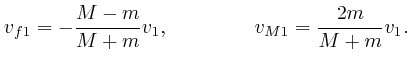
So if the 1 component of the velocity of a molecule of the ideal gas is ![]() at a particular time, then the only values the 1 component of the velocity of
that molecule ever takes are
at a particular time, then the only values the 1 component of the velocity of
that molecule ever takes are ![]() . If
. If ![]() , then that molecule
transfers momentum
, then that molecule
transfers momentum ![]() to the container wall at
to the container wall at ![]() , at moments
separated by time intervals
, at moments
separated by time intervals
![]() , so the average rate at which
that molecule transfers momentum to that container wall is
, so the average rate at which
that molecule transfers momentum to that container wall is
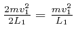 per unit time, so since force is the rate of change
of momentum, the average force exerted by that molecule on that container wall
is
per unit time, so since force is the rate of change
of momentum, the average force exerted by that molecule on that container wall
is
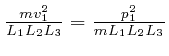
![]() in the outwards direction. Thus the pressure
in the outwards direction. Thus the pressure ![]() on
that container wall is the sum of
on
that container wall is the sum of
 over all the
gas molecules in the container.
over all the
gas molecules in the container.
From the formula above, integrated over the volume of the container, the most
likely number of molecules in a momentum bin centred at momentum ![]() , with
edge sizes
, with
edge sizes
![]() ,
,
![]() , and
, and
![]() , is:
, is:
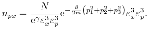
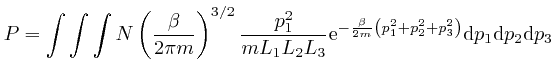
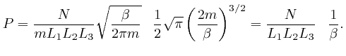
We'll assume now that this most likely number of molecules in each momentum
bin is the actual number of molecules in each momentum bin. Then the sum of
 over all the gas
molecules in the container is:
over all the gas
molecules in the container is:
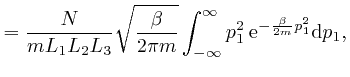
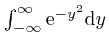
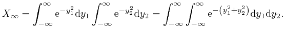
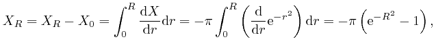
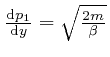
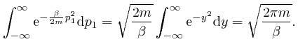
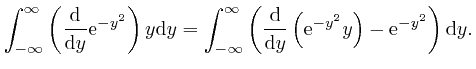
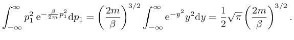
We'll calculate the above integral over ![]() by first calculating the
integral
by first calculating the
integral
 . We
found above that
. We
found above that
 , so:
, so:
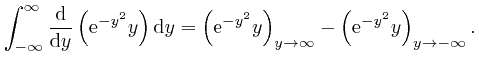
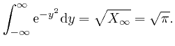
 , the magnitude of
 tends rapidly to 0 as
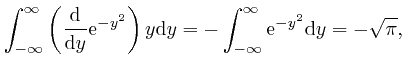
 , we have:

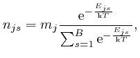
So if a system in thermal equilibrium at absolute temperature ![]() is composed
of a very large number microscopic objects of various types subject to
Newton's laws of motion, which we derived from de Maupertuis's principle of
stationary action in the previous post, here, and if the range of
possible positions and momenta of the objects is divided up into
is composed
of a very large number microscopic objects of various types subject to
Newton's laws of motion, which we derived from de Maupertuis's principle of
stationary action in the previous post, here, and if the range of
possible positions and momenta of the objects is divided up into ![]() tiny bins
of equal size, then from the result we found above, the most likely number of
objects of type
tiny bins
of equal size, then from the result we found above, the most likely number of
objects of type ![]() in position and momentum bin number
in position and momentum bin number ![]() is:
is:
One of the clues that led to the discovery of Dirac-Feynman-Berezin sums, and which made possible, among other things, the design and construction of the electronic device on which you are reading this blog post, came from the attempted application of the Boltzmann distribution to electromagnetic radiation. In the next post in this series, Electromagnetism, we'll look at the discoveries about electricity and magnetism that enabled James Clerk Maxwell, in the middle of the nineteenth century, to identify light as waves of oscillating electric and magnetic fields, and to calculate the speed of light from measurements of:
The software on this website is licensed for use under the Free Software Foundation General Public License.
Page last updated 4 May 2023. Copyright (c) Chris Austin 1997 - 2023. Privacy policy